Chapter 3: Goals and Rewards
How to Define Goals and Rewards?
INDEX
These are just my notes of the book Reinforcement Learning: An Introduction, all the credit for book goes to the authors and other contributors. My solutions to the exercises are on this page. Addtional concise notes for this chapter here.
We do not know what the rules of the game are; all we are allowed to do is watch the playing. Of course if we are allowed to watch long enough we may catch on a few rules. - Richard Feynman
3.1 The Agent-Environment Interface
In bandit problems we estimated the value \(q_*(a)\) for each action \(a\), in Markov Decision Process (MDPs) we estimate the value \(q_*(s, a)\) of each action \(a\) in each state \(s\). Or we estimate the value of each state given optimal action selection \(v_*(s)\). The agent and MDPs give rise to trajectory sequence like \(S_0, A_0, R_1, S_1, A_1, R_2...\). So the probability of given state-action pair is \[p(s',r|s,a)=Pr\{S_t=s', R_t=r \big| S_{t-1}=s, A_{t-1}=a\} \tag{1}\] \[\sum_{s'\in S}\sum_{r\in R}p(s',r|s,a) = 1\] Agent, Environment and Action are denoted in engineering terms as controller, controlled system (plant) and control signal respectively. Though you might feel that MDPs are not really used later because we almost have not information about them, we still use it to formalise our problem, to understand what the problems really are.
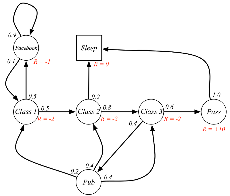
A sample Markov Decision Process
MARKOV PROPERTY: The probability of each possible value of \(S_t\) and \(R_t\) depends only on the immidiately preceeding step, that is all the information about all the aspects of past should be present in the given state. This gives rise to three different transition properties: \[p(s'|s,a) = \sum_{r\in R}p(s',r|s,a)\] \[r(s,a) \doteq \mathbb{E}[R_t|s,a] = \sum_{r\in R}r\sum_{s'\in S}p(s',r|s,a)\] \[r(s',a,s) \doteq \mathbb{E}[R_t|s',a,s] = \sum_{r\in R}r\frac{p(s',r|s,a)}{p(s'|s,a)}\] The general rule to follow is that anything that cannot be arbitrarily changed by the agent is condsidered to be outside of it and part of the environment.
Example 3.1: Bioreactor Suppose reinforcement learning is being applied to determine moment-by-moment tempratures and stirring rates for bioreactor (a large vat of nutrients and bacteria used to produce useful chemicals).
The states in this casre are likely to be thermocouple and other sensory readings, perhaps filtered and delayed, plus symbolic inputs representing the chemicals in the vat and the target chemicals. The actions then are tempratures and stirring rates for bioreactor.
Example 3.2: Pick and Place Robot Suppose reinforcement learning is being applied to control the motion of robot arm in a repetetive pick and place task.
The actions in this case might be the voltages applied to each motor at each joint, and the states might be the latest readings of joint angles and velocities
Example 3.3: Recyling Robot Read this from the book.
3.2 Goals and Rewards
REWARD HYPOTHESIS: All that we mean by the goal can be thought of as maximisation of expected value of cumulated sum of recieved scalar signals (called reward). Since the agent only learns from rewards, it is important that we set up rewards that truly indicate what we want accomplished.
The reward signal is our way of communicating to the robot what you want to achieve, not how you want to achieved.
3.3 Returns and Episodes
In general what we seek to maximise is the expected return, given by \(G_t\) for timesteps greater than \(t\). The tasks can be of two types, one with a clear end state called terminal state and those without. First considering only those episodes which end the expected reward can be calculated as \[G_t \doteq \sum_{t' = t}^{T}{R_{t'+1}} \tag{2} \] But this gets useless as \(T\to \infty\) because we cannot calculate the values for long episodes. This requires using of discounting, where we give less value to the later rewards using discount rate \(0 \leq \gamma \leq 1\) \[G_t \doteq \sum_{k=0}^{\infty}{\gamma^{k}R_{t+k+1}} \tag{3} \] A reward at \(k\) is only worth \(\gamma^{k-1}\) times what it would be worth if it was received immediately. Thus if \(\gamma=0\) the agent is "myopic" only concerned with immidiate reward. Returns at succesive steps can be combined to create a recursive format, this format is very useful in reinforcement learning. \[G_t \doteq R_{t+1} + \gamma R_{t+2} + \gamma^2 R_{t+3} + ...\] \[G_t = R_{t+1} + \gamma(R_{t+2} + \gamma R_{t+3} + ...)\] \[G_t = R_{t+1} + \gamma G_{t+1}\] This also works for all timesteps \(t < T\) even if the termination occurs at \(t+1\). Even if the reward is \(+1\) at each timestep even then we get a fixed reward \[G_t = \sum_{k=0}^{\infty}\gamma^k = \frac{1}{1-\gamma}\]
3.4 Unified Notation for Episodic and Continuing Tasks
Till now, we have discussed two kinds of reinforcement learning tasks, one in which the agent-environment interaction breaks down into a sequence of seperate episodes (episodic tasks), and one in which it does not (continuous tasks). Since we use these kinds of interactions throughout the book [and blogs], it is important to have consistency. We need to obtain a single notation that covers both episodic and continuing tasks.

Square block represents special absorbing state
We define returns as a sum over finite \((2)\) and infinite \((3)\) number of terms which can be unified by considering a special absorbing state, that transitions only to itself and returns reward \(0\). So the reward becomes \(+1, +1, 0, 0, ...\). This is useful because the sum of rewards with and without discounting remains the same. So we can modify \((3)\) to give \[G_t \doteq \sum_{k=0}^{\infty}{\gamma^{k}R_{t+k+1}} = \sum_{k = t+1}^{T}{\gamma^{k - t - 1}R_{t}} \tag{4}\] which works for \(T = \infty\) and \(\gamma = 1\). We use this convention throghout the book t oexpress close parallels between episodic and continuous tasks.
3.5 Polcies and Value Functions
Policy can be formally defined as mapping of state to probabilities of selecting each possible action, \(\pi(a|s)\) is the probability that \(A_t = a\) and \(S_t = s\) for any time step \(t\). Different reinforcement learning methods specify how agent's policy changes with experience. The value function of \(s\) under policy \(\pi\) is given as \(v_\pi(s)\) is the expected return when starting in \(s\) and following \(\pi\). For MDPs, it can be defined as follows \[v_\pi \doteq \mathbb{E}_{\pi}[G_t|S_t = s] \] \[= \mathbb{E}_{\pi}\left[\sum_{k = 0}^{\infty}{\gamma^k R_{t+k+1}\Big|S_t = s}\right] \tag{5}\] Similarly we define action-value function \(a\) as \(q_\pi(s,a)\) as expected return of starting in \(s\), taking action \(a\) and following \(\pi\) \[q_\pi(s,a) \doteq \mathbb{E}_{\pi}[G_t, S_t = s, A_t = a]\] \[= \mathbb{E}_{\pi}\left[\sum_{k = 0}^{\infty}{\gamma^k R_{t+k+1}\Big|S_t = s, A_t = a}\right] \tag{6}\]
From exercises \(3.12\) and \(3.13\) we get values \[v_\pi(s) = \sum_{a \in \mathbb{A}(s)}{\pi (a|s) q_\pi(s,a)} \tag{7}\] \[q_\pi(s,a) = \sum_{s' \in S}\sum_{r \in \mathbb{R}}{p(s',r|s,a)v_\pi(s)} \tag{8}\] The value functions \(v_\pi\) and \(q_\pi\) can be estimated from experience. Monte Carlo Problems: So if we calculate the average value of the state it would converge to \(v_\pi(s)\) as the number of samples reaches \(\infty\). And if we keep seperate average of each value of state and actions encountered the number reaches to \(q_\pi(s,a)\). We can train the agent to maintain a parameterised average as functions with fewer parameters than states. This approach is called parameterised function approximators, and dicuss this later.
The most important property to use is the recursive nature of value functions. For any policy \(\pi\) and state \(s\), the following consistency holds true: \[v_\pi(s) \doteq \mathbb{E}[G_t|S_t = s]\] \[= \mathbb{E}[R_{t+1} + \gamma G_{t+1} | S_t = s]\] \[= \sum_{a} \pi(a|s) \sum_{s', r} p(s',r|s,a) \left[r + \gamma\mathbb{E}[G_{t+1} | S_{t+1} = s']\right]\] \[= \sum_{a} \pi(a|s) \sum_{s', r} p(s',r|s,a) \left[r + \gamma v_\pi(s')\right] \tag{9}\] where it is implicit that \(s \in S\) (or \(S^+\) for episodic problem), \(r \in \mathbb{R}\) and \(a \in \mathbb{A}(s)\). Note how \((9)\) can be read as a expectation value, as it sums over 3 variables \(s'\), \(r\) and \(a\). For each triple we weight using its probability as \(\pi(a,s)p(s',r|s,a)\) and sum it over all possibilities to calculate the expected value. Equation \((9)\) is Bellman Equation for \(v_\pi\). Which states that the value of start state must equal (discounted) value of the expected next state plus the reward expected along the way.
We define this using backup diagrams where states are represented using open circles and actions using sold circles. Starting state is \(s\) and we use policy \(\pi\) and take action \(a\), obtaining reward \(r\) and reaching state \(s'\) depending on dynamics \(p\).
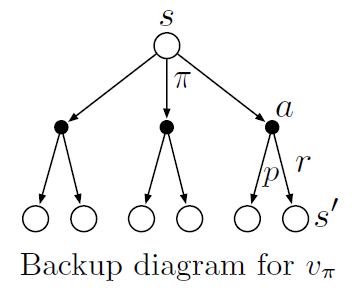
Example of backup diagram for \(v_\pi\)
The value function \(v_\pi\) is the unique solution to Bellman equation. These operations transfer value information back to state or state-action pairs from its successor states or state-action pairs respectively. Note that though unlike state transition graphs the output state can be same as the input state i.e. distinct states in backup diagram do not represent distinct states as in state transition graphs.

Grid World for the example 3.5
Example 3.5: Gridworld We are given a gridworld as shown above, where the agent can move around in north, south, east, west. It gets reward \(-1\) for actions that take it off grid, \(+10\) and \(+5\) for those that move out of special states \(A\) to \(A'\) and \(B\) to \(B'\) respectively and \(0\) everywhere else. The chart on the right are the value for the states. Notice negative values near the edge as agent is more likely to get off grid. Notice that the value at \(A\) is less than \(10\) as at \(A'\) it is likely to go off grid, whereas the value at \(B\) is more that \(5\) as it is safer at \(B'\).

Golf World for the example 3.6
Example 3.6: Golf We are given a task to convert Golf into a reinforcement learning problem. So we need to do define what the states,actions and rewards are. For this the reward is \(-1\) for each hit and \(0\) for completing taksk and \(-\infty\) for being is sand because ball can never be removed from sand. The actions then become angle, speed and which club to use. For simplicity assume our action is only to select the club to use. with putt we can only hit so far and so the state-value function then becomes \(v_{putt}\) and it shown in the above state diagram. If we use driver instead of putt then we need to know the location to hit at and so the action-value function \(q_*(s, driver)\) and is given in the lower diagram.
The value of state \(v(s)\) depends upon the values of action possible in the given state and how likely the given each action can be taken under current policy. The value of action \(q(s,a)\) depends on expected next reward and sum of expected next rewards. From examples \(3.18\) and \(3.19\) we get \[v_\pi(s) = \sum_{a \in A} \pi(a|s) q_\pi(s,a) \tag{10}\] \[q_\pi(s,a) = \sum_{s',r} p(s',r|s,a)\left[r + \gamma v_\pi(s') \right] \tag{11}\]
3.6 Optimal Policies and Optimal Value Functions
A policy \(\pi\) is defined to be better than or equal to policy \(\pi'\) if its expected returns are greater than or equal to that of \(\pi'\) for all states i.e. \(\pi \geq \pi'\) iff \(v_\pi(s) \geq v_{\pi'}(s) \forall s \in S\). However there is one policy that is better than or equal to all other policies, this is called Optimal Policy denoted by \(\pi_*\). They share same state value function denoted by \(v_*\) \[v_*(s) \doteq \max_\pi v_\pi(s) \forall s \in S\] They also share the same action value function denoted by \(q_*\) \[q_*(s,a) \doteq \max_\pi q_\pi(s,a) \forall s \in S, a \in A(s)\] We can write \(q_*\) in terms of \(v_*\) as follows \[q_*(s,a) = \mathbb{E}\left[R_{t+1} + \gamma v_*(S_{t+1}) | S_t = s, A_t = a \right]\]
Example 3.7: Optimal Value Functions for Golf The optimal action-value function gives values after commiting to a particular first action. Read complete from book.
Bellman equations need to be modified for use with optimal functions as optimal state value function \(v_*\) must satisfy self-consistency. The modified equation for \(v_*\) is called Bellman Optimality Equation \[v_*(s) = \max_{a \in A(s)}q_{\pi_*}(s,a)\] \[= \max_{a} \mathbb{E}_{\pi_*}\left[ G_t | S_t = s, A_t = a\right]\] \[= \max_{a} \mathbb{E}_{\pi_*}\left[ R_{t+1} + \gamma G_{t+1} | S_t = s, A_t = a\right]\] \[= \max_{a} \mathbb{E}_{\pi_*}\left[ R_{t+1} + \gamma v_{*}(S_{t+1}) | S_t = s, A_t = a\right] \tag{12}\] \[= \max_{a} \sum_{s', r}p(s',r|s,a) \left[ r + \gamma v_{*}(s')\right] \tag{13}\] Here the last two equations \((11, 12)\) form Bellman optimality equation for \(v_*\). The Bellman optimality for \(q_*\) is given as \[q_*(s,a) = \mathbb{E} \left[R_{t+1} + \gamma \max_{a'} q_*(S_{t+1}, a') \big| S_t = s, A_t = a \right]\] \[= \sum_{s',r} p(s',r|s,a) \left[r + \gamma \max_{a'}q_*(s',a')\right] \tag{14}\] We will also need to modify the backup diagrams, here the arcs represent the maximum over the choice taken. The diagram on left and right represent \((12)\) and \((13)\) respectively.

New backup diagrams for \(v_*\) and \(q_*\)
It is easy to find solution for finite MDPs as it is independent of policy. If we know the dynamics of environment \(p\) then we can in theory, calculate the optimal value function \(v_*\) as the MDP breaks into \(n\) equations for \(n\) states. Then we can select any method to solve non-linear equation. In turn we can solve to find optimal action value function \(q_*\). For each state \(s\), there will be one or more actions at which the maximum is obtained in the Bellman optimality equation. Any policy that assigns non-zero probability only to those actions is an optimal policy.
So if we have the optimal policy then we can take the best action for each state and it becomes a one step search or Greedy Search. The beauty of \(v_*\) is that if one uses it to evaluate the short term consequences to actions specifically, the one-step consequences, then a greedy policy is actually the optimal policy as \(v_*\) accounts for the reward consequences of all possible future behaviour. Having \(q_*\) means that agent doesn't even have to do search but instead simply select action that maximises \(q_*(s,a)\).
Example 3.9 Bellman Optimality Equations for Recycling Robot In example 3.3 we look at a robot with the following MDP. We need to calculate the Bellman optimality equations for the same

MDP for examples 3.3 and 3.9
We use the notation \(high (h)\) and \(low (l)\) for states and \(search (s)\), \(wait (w)\) and \(recharge (re)\). To calculate the \(v_*\) we use \((13)\), for \(v_*(h)\) we have actions \(s\) and \(w\). So we get the equations \[q(h,s) = p(h|h,s)[r(h,s,h) + \gamma v_*(h)] + p(l|h,s)[r(h,s,l) + \gamma v_*(l)] \] \[q(h,w) = p(h|h,w)[r(h,w,h) + \gamma v_*(h)] + p(l|h,w)[r(h,w,l) + \gamma v_*(l)] \] \[v_*(h) = \max \begin{cases} q(h,s) \\ q(h,w) \end{cases} \] \[v_*(h) = \max \begin{cases} r_s + \gamma\left[ \alpha v_*(h) + (1 - \alpha)v_*(l)\right] \\ r_w + \gamma v_*(h) \end{cases} \] Similarly for value of \(low\) state, \(v_*(l)\) we have three actions \(s\), \(w\) and \(re\). Using the above method we obtain the value \[v_*(l) = \max \begin{cases} \beta r_s - 3(1- \beta) + \gamma \left[(1 - \beta)v_*(h) + \beta v_*(l) \right] \\ r_w + \gamma v_*(l) \\ \gamma v_*(h) \end{cases}\]
There are three main factor that prevent solving for Bellman optimality equation
Many different decision making methods can be viewed as as ways of approximately solving the Bellman optimality equation. For example, heuristic search methods can be viewed as expanding the right side of \((13)\) several times upto some depth, forming a "tree" of possibilities, and then using a heuristic evaluation function to approximate \(v_*\) at the "leaf" nodes. The methods of dynamic programming can be related even more closely.
The undiscounted formulation is appropriate for episodic task, in which agent-environment interaction breaks natuarally into episodes; the discounted formulation is appropriate for continuous tasks, in which inteaction does not naturally break into episodes but continues without limit.