Chapter 3 Exercises
Some solutions might be off
NOTE: This part requires some basic understading of calculus.
These are just my solutions of the book Reinforcement Learning: An Introduction, all the credit for book goes to the authors and other contributors. Complete notes can be found here. If there are any problems with the solutions or you have some ideas ping me at bonde.yash97@gmail.com.
3.1 Types of MDP
I would like to divide the types of MDP based on the state action forms.
3.2 Is MDP framework sufficient
Goal oriented learning tasks are those tasks where a goal is learnt, the learning occurs using rewards which are given for each state and action. One problem is when there are multiple rewards and the goal is achieved using one combination. This makes traversing MDP difficult and in turn inadequate for representation in MDP. Another example is when the states are difficult to comprehend or proper state representation is not possible.
3.3 Fine Lines in MDP
The fine line is the line of actions. Agents and environment seperate where we can obtain the given staet and take actions to influence that state. THe depth on the other hand is the scale of the problem we are solving. A car is agent as it controls accelerator, stearing angle and brake, while is moves around in the environment. While a logistics software operating large fleets would concern itself with different problem and thus its actions are not acceleration or stearing angle. One location of line is preffered over the other looking at and depending upon the problem being solved, there are certain constraints:
3.6 Pole Balancing (Episodic vs. Continuous)
When we get reward \(-1\) at moment of failure and zero everywhere else, we can see that the return obtained as episodic and discounted case is \(-\gamma^K\) where \(K\) is the time step at which failure occurs. When we consider this as a continuous and discounted we see that rewards would vary widely, and in case of terminal failure (when system cannot recover) it keeps returning large negative values while learning is not really possible.
3.7 Maze Runner
In any maze we get reward \(+1\) for completing the maze. In larger mazes the probability of completing the maze tends to \(0\) and so the rewards recieved become very sparse. This results in learning showing no improvement in escaping the maze. We have not effectively communicated to the agent what we want.
3.8 Returns Numerical
The trick is to calculate from the end and proceed to start using formula \(G_t = R_{t+1} + \gamma G_{t+1}\). So we start by calculating \(G_5 = 0\), \(G_4 = R_5 + \gamma G_5\) and so on. So we get the values \(G_0 = 2, G_1 = 6, G_2 = 8, G_3 = 4, G_4 = 2, G_5 = 0\).
3.9 Returns Numerical
Given that \(R_1 = 2\) and rest of the sequence is infinitely long with reward at each step being \(7\), trick is to calculate the later return first (\(G_1\) then \(G_0\)). This is a simple sum of geometric progression as \[G_1 = \sum_{k = 0}^{\infty}\gamma^k R_{1 + k + 1}\] \[G_1 = \frac{7 \times (1 - \gamma)^\infty}{1 - \gamma}\] \[G_1 = \frac{7}{0.1} = 70\] and using the formula \(G_0 = R_1 + \gamma G_1\) we get value \(G_0 = 2 + 0.9 \times 70 = 65\).
3.10 Returns Numerical
Sum of basic geometric progression.
3.11 Expected Return
Given that current state is \(s = S_t\) and action probability distribution is \(\pi(a|s)\), so calculate the expectation for \(R_{t+1}\) in terms of \(\pi\) and \(p(s',r|s,a)\). \[\mathbb{E}_\pi[R_{t+1}|S_t = s, A_t = \pi(a|s)]\] \[= \sum_{r\in\mathbb{R}} p(s', r| s, \pi(a|s))\]
3.12 Equation for \(v_\pi\) in terms of \(q_\pi\) and \(\pi\)
Equation can be given as \(v_\pi(s) = \sum_{a \in \mathbb{A}(s)}{\pi (a|s) q_\pi(s,a)}\)
3.13 Equation for \(q_\pi\) in terms of \(v_\pi\) and four argument \(p\)
Equation can be given as \(q_\pi(s,a) = \sum_{s' \in S}\sum_{r \in \mathbb{R}}{p(s',r|s,a)[r + v_\pi(s')]}\)
3.14 Value of Centre Tile

Grid World for the problem
We are given values \(+2.3\), \(+0.4\), \(-0.4\) and \(+0.7\) of N,E,S,W respectively, reward at each state is \(r = 0\) and \(\gamma = 0.9\). We know from \((9)\) that, and we are supposed to ue this to calculate the value of centre tile. \[v_\pi(s)= \sum_{a} \pi(a|s) \sum_{s', r} p(s',r|s,a) \left[r + \gamma v_\pi(s')\right]\] Now since this is the centre tile transition probability \(p(s',r|s,a) = 1\) and so we get \[v_\pi(s) = \sum_{a}\pi(a|s) \gamma (\sum_{s'} v_\pi(s'))\] \[v_\pi(s) = \sum_{a}{\pi(a|s)\gamma \times 3}\] \[v_\pi(s) = \sum_{a}{\pi(a|s) \times 2.7}\] As this is the expected value and policy follows a random actions, the final value will simply be the mean of \(2.7\). Thus we get \(v_\pi(centre) = \frac{2.7}{4} \approx +0.7\).
3.15 Adding Constant to each Reward
In the given example rewards are positive for goals, negative for running out of world and \(0\) everywhere else. No, signs of the reward does not matter, if we take a simple case and flip the values, such that positive rewards are not negative rewards and vica versa we get \[v'_\pi(s) = \mathbb{E}_\pi\left[{\sum_{k=0}^{\infty} {\gamma^k (-R_{t+k+1})} \big| S_t = s} \right]\] \[v'_\pi(s) = -v_\pi(s) \] So we also get \(q_\pi(s,a)\) as \[q'_\pi(s,a) = \sum_{s' \in S}\sum_{r \in \mathbb{R}}{p(s',r|s,a) v'_\pi(s)}\] \[q'_\pi(s,a) = - \sum_{s' \in S}\sum_{r \in \mathbb{R}}{p(s',r|s,a) v_\pi(s)}\] \[q'_\pi(s,a) = - q_\pi(s,a)\] So we only have to change the decision making method. Moving to second part of the question, if we add a constant \(c\) to all the rewards in \((4)\) we get value \[G'_t = \sum_{k=0}^{\infty}{\gamma^{k}(R_{t+k+1} + c)}\] \[G'_t = G_t + c\sum_{k=0}^{\infty}{\gamma^{k}} \] \[v'_\pi(s) = \mathbb{E}_\pi\left[G'_t | S_t = s \right]\] \[ = \mathbb{E}_\pi\left[G_t + \frac{c}{1 - \gamma} \big| S_t = s \right] \tag{1}\] The value of the expectation only shift when we add any constant value to it, so the relative values remain the same and there is no difference. Expanding \((1)\) \[v'_\pi(s) = \sum_{a}\pi(a|s)\sum_{s',r}p(s',r|s,a)\left(r + c + \gamma v'_\pi(s')\right)\] \[= \sum_{a}\pi(a|s)\sum_{s',r}p(s',r|s,a)\left(r + \gamma v_\pi(s') + c + \frac{\gamma c}{1 - \gamma}\right)\] \[= v_\pi(s) + \frac{c}{1- \gamma}\sum_{a}\pi(a|s)\sum_{s',r}p(s',r|s,a) \] \[v'_\pi(s) = v_\pi(s) + v_c\] So the constant value added to each state \(v_c = \frac{c}{1 - \gamma}\).
3.16 Adding Constant to each Reward (for episodic task)
Adding a constant \(c\) to each reward in an episodic task such as maze runner, should improve the results as the rewards are not longer very sparse. In the original setting the learner got \(+1\) reward for completing the maze and \(0\) everywhere else. This resulted in sparse rewards prohibiting it to learn very less. But in order to prove this, it should be generalisable to every episodic task.
3.17 Bellman Equation for action value

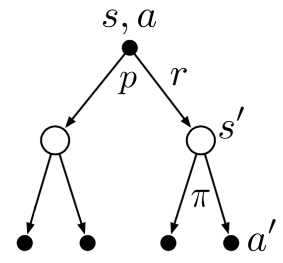
Backup Diagram for \(q_\pi\)
Derive bellman equation for action-value pair \((s,a)\) from the backup diagram given above. It can be derived as follows \[q_\pi(s,a) = \mathbb{E}_\pi\left[G_t | S_t = s, A_t = a \right]\] \[= \mathbb{E}_\pi\left[R_{t+1} + \gamma G_{t+1} | S_t = s, A_t = a \right]\] Note that for any backup diagram multiply the transition probability \(p(s',r|s,a)\) with the expectation of rewards. Also \(\mathbb{E}[R_{t+1} + \gamma G_{t+1}|...] = \mathbb{E}[R_{t+1}|...] + \gamma\mathbb{E}[G_{t+1}|...]\) \[= \sum_{s',r} p(s',r|s,a) \left[\mathbb{E}_\pi[R_{t+1}| S_t = s', A_t = a'] + \gamma\mathbb{E}[G_{t+1}|S_t = s', A_t = a']\right]\] \[= \sum_{s',r} p(s',r|s,a) \left[r + \gamma \sum_{a'}\mathbb{E}[G_{t+1}|S_t = s']\right]\] Note that \(\sum_{a'}\mathbb{E}[G_{t+1}|S_t = s'] = v(s)\) and \(\mathbb{E}_\pi[R_t|...] = r\) where \(...\) can be any set of conditional parameters. \[q_\pi(s,a)= \sum_{s',r} p(s',r|s,a) \left[r + \gamma \sum_{a'}\pi(a'|s')q_\pi(s',a')\right]\]
3.18 Bellman Equation from backup diagram

Backup diagram for example 3.18
For the three possible actions let \(A = \{a_1, a_2, a_3\}\) or set of all actions. \[v_\pi(s) = \mathbb{E}_\pi\left[G_t | S_t = s \right]\] \[v_\pi(s) = \sum_{a \in A} \pi(a|s) q_\pi(s,a)\]
3.19 Bellman Equation from backup diagram

Backup diagram for example 3.19
The action value \(q(s,a)\) depends on expected next reward and expected sum of remaining rewards. Writing in terms of expectation we get \[q_\pi(s,a) = \mathbb{E}_\pi\left[G_t | S_t = s, A_t = a\right]\] For all branches we get values as follows \[q_{\pi}^{1}(s,a) = p(s_1,r_1|s,a)\left[r_1 + \gamma v_\pi(s_1) \right]\] \[q_{\pi}^{2}(s,a) = p(s_2,r_2|s,a)\left[r_2 + \gamma v_\pi(s_2) \right]\] \[q_{\pi}^{3}(s,a) = p(s_3,r_3|s,a)\left[r_3 + \gamma v_\pi(s_3) \right]\] The final value will be sum of the three \[q_\pi(s,a) = q_{\pi}^{1}(s,a) + q_{\pi}^{2}(s,a) + q_{\pi}^{3}(s,a)\] \[ = \sum_{s',r} p(s',r|s,a)\left[r + \gamma v_\pi(s') \right]\]
3.22 Bellman Equation from backup diagram

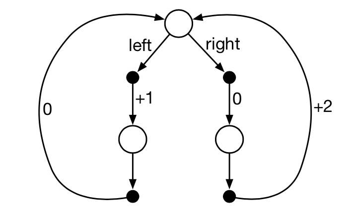
MDP for for example 3.19
Given that there are only two deterministic policies \(\pi_{left}\) and \(\pi_{right}\) and decision has to be taken only at the top state, what are the optimal policies when \(\gamma = 0, 0.9, 0.5\). We calculate this using the returns \(\gamma = 0; \pi_* = \pi_{left}; r = +1\), \(\gamma = 0.09; \pi_* = \pi_{right}; r = +1.8\) and \(\gamma = 0.5; \pi_* = None; r = +1\) in either case.
3.23 Action Value Bellman Equation for Robot
From example 3.9 we know the values for \(v(h)\) and \(v(l)\) can be given as \[v(h) = \pi(s|h)q(h,s) + \pi(w|h)q(h,w)\] \[v(l) = \pi(s|l)q(l,s) + \pi(w|l)q(l,w) + \pi(re|l)q(l,re)\] Similarly we calculated the action values \(q\) as \[q(h, s) = r_s + \gamma\left[ \alpha v(h) + (1 - \alpha)v(l)\right]\] \[q(h, w) = r_w + \gamma v(h)\] \[q(l, s) = \beta r_s - 3(1- \beta) + \gamma \left[(1 - \beta)v(h) + \beta v(l) \right]\] \[q(l, w) = r_w + \gamma v(l)\] \[q(l, re) = \gamma v(h)\] Combining these, we can get the bellman equations for action-value functions.
3.25 Equation for \(v_*\) in terms of \(q_*\)
\[v_*(s) = \max q_*(s,a)\]
3.26 Equation for \(q_*\) in terms of \(v_*\)
\[q_*(s,a) = \max p(s',r|s,a)v_*(s)\]
3.27 Equation for \(\pi_*\) in terms of \(q_*\)
\[\pi(a|s) = \max_a q_*(s,a)\]
3.28 Equation for \(\pi_*\) in terms of \(v_*\) and for-argument \(p\)
\[\pi(a|s) = \max_a \sum_{s',r} p(s',r|s,a)[r + \gamma v_*(s)]\]