Chapter 5: Monte Carlo Methods

Learning from experience

INDEX

These are just my notes of the book Reinforcement Learning: An Introduction, all the credit for book goes to the authors and other contributors. My solutions to the exercises are on this page. Addtional concise notes for this chapter here. There is also a Deepmind's Youtube Lecture and slides for model free value extimation and model free control. Some other slides.

We do not know what the rules of the game are; all we are allowed to do is watch the playing. Of course if we are allowed to watch long enough we may catch on a few rules. - Richard Feynman

Introduction

Unlike previous chapter, we do not assume full knowledge of probability distributions of transitions, Monte Carlo methods only require experience - sample knowledge of states, actions and rewards. It can learn from actual experiences, despite having no prior knowledge of environments dynamics and from stimulated experience, altough model is required it needs only the sample transitions.

The term "Monte Carlo" is often used more broadly for any estimation method whose operations involves a significant random component. Here we use it more specifically for methods based on averaging complete returns. This can be considered a bandit problem except that here all the bandits (states) are related. To handle the non-stationarity we adapt the idea of general policy iteration (GPI) as seen previously.

Monte Carlo methods are good for episodic tasks because they have a simple idea that value of anything is simply the returns that it gets, thus the episode must always end.

5.1 Monte Carlo Predictions

The value function stabilizes only when it is consistent with the current policy, and the policy stabilizes only when it is greedy with respect to the current value function. Thus both the processes stabilize only when a policy has been found which is greedy with respect to its own evaluation functions. This implies that Belmann optimality equation holds adn thus that the policy and value function are optimal. In either case, the two processes together achieve the overall goal of optimality even though neither is attempting to achieve it directly.

The goal here is to learn value function for some policy \(v_\pi\) from episodes of experience under \(\pi\) \[S_1, A_1, R_2, ... ~ \pi\] and instead of having an expected return \(v_\pi = \mathbb{E}[G_t | S_t = s]\) we use emperical mean.

First visit MC only considers each state once in an episode and take mean from that point onwards we do not consider if in some loop we visit that state again. We get the optimal value function from the law of large numbers and keep on averaging them over multiple episodes. Every visit MC increments the state counter every time I visit that state and not only once per episode.

We can perform incremental averaging which allows us to perform online learning. It basically means that "new me is old me plus some step size". We can write in in the iterative format as, for each state \(S_t\) with return \(G_t\) \[N(S_t) = N(S_t) + 1\] \[V(S_t) = V(S_t) + \alpha(G_t - V(S_t))\] Where \(\alpha = 1/N(S_t)\) (step-size) for stationary distribution and is some value for non-stationary distribution for running mean, i.e. forget old episodes so we don't have the baggage of past.

5.2 Monte Carlo Estimation of Action Values

When there is model available we can simply perform next state lookup and choose action that brings to state that has best value. However when there is not state value available then we must get estimates for action-value pairs, thus one of the primary goals of Monte Carlo estimation is to calculate \(q_*\). Just like for value estimation we can have first-visit MC and every-visit MC.

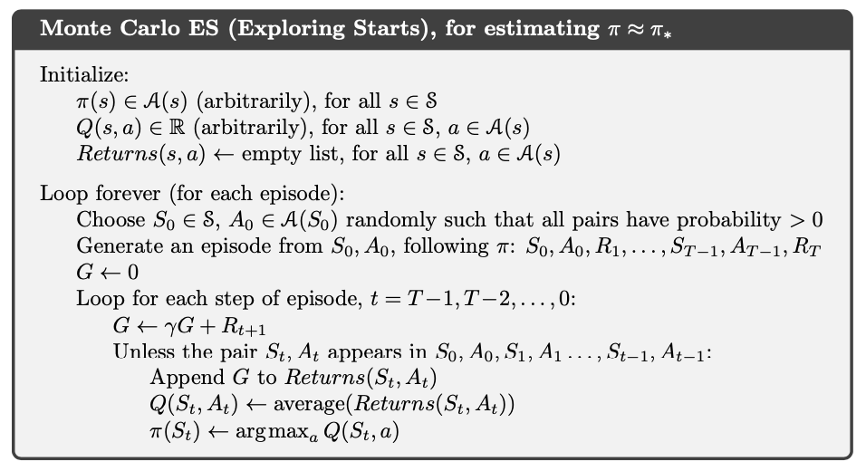
One serious problem we face is that there will be many state-action pairs that will never be visited and in order to compare we need to estimate the value of all possible actions in a state. One solution is to give each state a starting non-zero probability of being selected in the start. Thi guarantees that all state-action pairs will be visited an infinite number of times in the limit of infinite number of episodes. We call this assumption exploring starts.

5.3 Monte Carlo Control

It follows the general principle laid in Policy Iteration where we loop evaluation followed by greedy policy but instead of having plain value function we have action-values.

Since no model is required we can make policy by simply taking argmax of action-values \[\pi(s) \doteq argmax_a q(s,a)\] We can use this as a guarantee to convergence as \[q_{\pi_k}(s, \pi_{k+1}(s)) = q_{\pi_k}(s, argmax_a q(s,a)) \] \[= \max_a q_{\pi_k}(s,a)\] \[\geq q_{\pi_k}(s, \pi_k(s))\] \[\geq v_{\pi_k}(s) \] But this assumes two things, one that episodes have exploring starts and other that we infinite number of episodes. To obtain a practical algorithm we'll have to remove both the assumptions.

There are two approaches for getting this working, first the vannila approach. One is to holf firm to the idea of approximating \(q_{\pi_k}\) in each policy evaluation. Measurements and assumptions are made to obtain bounds on the magnitude and probability error in the estimates, and then sufficient steps are taken during each policy evaluation. However, it is also to require far too many episodes to be useful in practice on any but the smallest problems.

It is easy to see that MCES cannot converge to a suboptimal policy. If it did, then the value function would eventually converge to the value function of that policy and that in turn would cause the policy to change. Though practically demonstrated, it has not beenproven as a theory and is on of the most fundamental open theoretical questions in reinforcement learning.q

5.4 Monte Carlo Control without Exploring Starts (On-Policy)

There are two appraoches to ensuring this, resulting in what we call on-policy methods (evaluate or improve the policy that is used to make decisions) and off-policy methods (evaluate or improve a policy different from that used to generate data). Here we discuss the on-policy MC control w/o exploring starts.

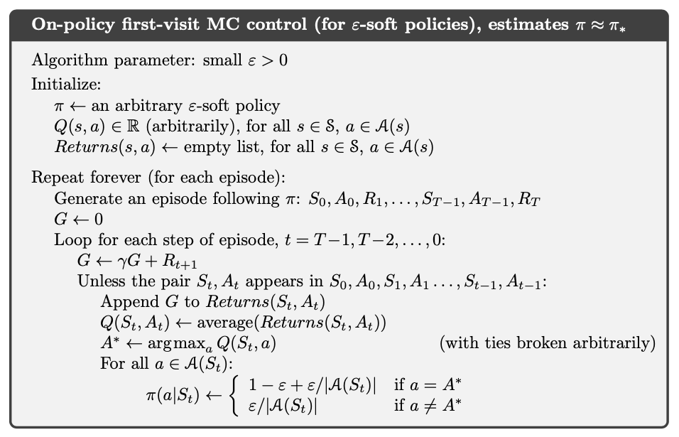
In on-policy control methods we have a soft policy, meaning that \(\pi(a|s) > 0\) for all \(s \in S\) and all \(a \in A(s)\), but gradually shift to deterministic optimal policy. The on-policy algorith that we chose here is \(\epsilon-greedy\) that is it takes the maximal estpimated action value but with probabilty \(\epsilon\) they take a radom action. We use a subset of \(\epsilon-greedy\) called \(\epsilon-soft\) in which the minimal probability of selection is \(\pi(a|s) \geq \frac{\epsilon}{|A(s)|}\) and the remaining bulk of the probability \(1 - \epsilon + \frac{\epsilon}{|A(s)|}\) is given to greedy action. Fortunately, GPI does not require that policy be taken all the way to greedy policy, only that it be moved toward a greedy policy.

We can show that \(\epsilon-greedy\) w.r.t. to \(q_\pi\) is an improvement over any \(\epsilon-soft\) policy using the policy improvement theorem. Let \(\pi'\) be the \(\epsilon-greedy\) policy as \[q_\pi(s, a) = \sum_{a} \pi'(a|s) q_\pi(s,a)\] \[ = \frac{\epsilon}{|A(s)|}\sum_{a}q_\pi(a,s) + (1-\epsilon)\max_a q_pi(s,a)\] The sum of a weighted average with non-negative weights summing 1 is less than equal to the largest number averaged. As \(\pi(a,s_t) = 1 - \epsilon + \frac{\epsilon}{|A(s)|}\) we can also write it as \(\frac{\pi(a|s) - \frac{\epsilon}{|A(s)|}}{1 - \epsilon} = 1\) and use this as averaging over all the actions \[\geq \frac{\epsilon}{|A(s)|}\sum_{a}q_\pi(a,s) + (1-\epsilon) \sum_{a}\frac{\pi(a|s) - \frac{\epsilon}{|A(s)|}}{1 - \epsilon} q_\pi(s,a)\] \[= \sum_{a}\pi(a|s)q_\pi(s,a) = v_\pi(s)\] Thus by the policy improvement theorem, \(\pi' \geq \pi\) (i.e. \(v_{\pi'}(s) \geq v_\pi(s)\) for all \(s \in S\))

If we now push this random action into environment we get the optimal policies as \(\hat{v_*}\) and \(\hat{q_*}\) then we can write as follows \[\hat{v_*}(s) = (1 - \epsilon)\max_a \hat{q_\pi}(a,s) + \frac{\epsilon}{|A(s)|}\sum_a\hat{q_*}(s,a)\] \[= (1 - \epsilon)\max_a \sum_{s',r}p(s',r|s,a)[r + \gamma \hat{v_*}(s'))] \\ + \frac{\epsilon}{|A(s)|}\sum_a \sum_{s',r}p(s',r|s,a)[r + \gamma \hat{v_*}(s'))] \] We know from above that \[v_\pi(s) = \frac{\epsilon}{|A(s)|}\sum_{a}q_\pi(a,s) + (1-\epsilon)\max_a q_pi(s,a)\] \[= (1 - \epsilon)\max_a \sum_{s',r}p(s',r|s,a)[r + \gamma v_\pi(s'))] \\ + \frac{\epsilon}{|A(s)|}\sum_a \sum_{s',r}p(s',r|s,a)[r + \gamma v_\pi(s'))]\] The above two equations are same except that \(\hat{v_*} \rightarrow v_\pi\) and if the two values are same then \(v_\pi = \hat{v_*}\), i.e. we have reached the optimal policy.

Thus we have showed that there will be continual improvements in every step iff we already are not at the optimal value function. This brings us to roughly the same point as in the previous section only that we achieve best policy among \(\epsilon-soft\) policies, but on the other hand we have elimited the assumption of exploring starts.

5.5 Off-policy Prediction via Importance Sampling

All learning control methods face a dilemma: they seek to lean optimalaction values condional to subsequent optimal behaviour, but they need to behave non-optimally ni order to explore all actions (to find optimal actions). The straightforward approach is to use two separate policies, one that the is learned about and that becomes the optimal policy, and one that is more exploratory and is used to generate behaviour. This is called off-policy learning.

Say that we want to calculate \(v_\pi\) and \(q_\pi\) and we have target policy \(\pi\) and behaviour policy \(b\), where \(b \neq \pi\). In order to use episoldes from \(b\) to estimate values for \(\pi\), we require that every action taken under \(\pi\) be occasionally taken under \(b\). This makes the \(\pi\) deterministic and greedy according to the action-state value i.e. more optimal, while the behaviour policy \(b\) remains stochastic in some states, more exlporatory.

Almost all off-policy algorithms use importance sampling, which is used to estimate expected values under one distribution given samples from the another. Given a starting state \(S_t\), the probability of the subsequent state-action trajectory \(A_t, S_{t+1}, A_{t+1}, ... ,S_T\), occuring under policy \(\pi\) \[P\{A_t, S_{t+1}, A_{t+1}, ... ,S_T | S_t, A_{t:T-1} ~ \pi\}\] \[= \pi(A_t|S_T)p(S_{t+1}|S_t, A_t)\pi(A_{t+1}, S_{t+1}) \cdot\cdot\cdot p(S_T|S_{T-1}, A_{T-1})\] \[= \Pi_{k=t}^{T-1} \pi(A_k|S_k)p(S_{k+1}|S_k, A_k)\] where \(p\) is the state-transition function. Now we can calculate the importance sampling ratio as \[\rho_{t:T-1} \doteq \frac{\Pi_{k=t}^{T-1} \pi(A_k|S_k)p(S_{k+1}|S_k, A_k)}{\Pi_{k=t}^{T-1} b(A_k|S_k)p(S_{k+1}|S_k, A_k)}\] \[= \Pi_{k=t}^{T-1} \frac{\pi(A_k|S_k)}{b(A_k|S_k)}\] Thus this is independent of the MDP and it's transition functions instead depends only on the two policies. Now we know \(v_b(s) = \mathbb{E}[G_t|S_t = s]\) to get the value for any state using policy \(\pi\) we multiply the return by importance sampling ratio as \[v_\pi(s) = \mathbb{E}[\rho_{t:T-1}G_t | S_t = s]\]

Now we are ready to perform MC algorithm that averages return from a batch of observed episodes following policy \(b\) to estimate \(v_\pi(s)\), again we can use both every-visit and first-visit MCE. We define the set of all time steps in which state \(s\) is visted \(J(s)\). For every-visit MCE it is convinient to have time series that cross the episode boundaries, so if state terminates at \(t = 100\), next state will start from \(t = 101\). For a first-visit, \(J(s)\) would only include time steps that were visits to \(s\) in that episode.

Let \(T(t)\) denote the first time of termination following time \(t\), and \(G_t\) denote the return after \(t\) up through \(T(t)\). Then \(\{G_t\}_{t \in J(s)}\) are returns pertaining to state \(s\) and \(\{\rho_{t:T(t)-1}\}_{t \in J(s)}\) are the corresponding importance sampling ratios. So we can calculate Ordinary Imporance Sampling \[V(s) \doteq \frac{\sum_{t\in J(s)}\rho_{t:T(t) - 1}G_t}{|J(s)|}\] and Weighted Imporantance Sampling as \[V(s) \doteq \frac{\sum_{t\in J(s)}\rho_{t:T(t) - 1}G_t}{\sum_{t\in J(s)}\rho_{t:T(t) - 1}}\] or zero if the denominator is zero.

To better understand the difference assume that we run for just one step and calculate the value estimates. The weighted one will return same value as \(v_b\) as \(\rho\) terms cancel each other, in a way we call this bias. The ordinary will return the \(v_b\) times the sampling ratio. Imagine that the sampling ratio was \(10\) then the estimate would be ten times, which is far from actual sample. Thus we can summarise as follows "Oridinary has no bias but high variance and Weighted has bias but variance \(\leq 1\), though bias asymptotically reaches to zero".

In practice the weighted estimator has dramatically lower variance and is strongly preffered also every-visit algorithms are used becuase it removes the need to maintain which states have been visited.

Example 5.4 This question is used to evaluate this state: "the dealer is showing deuce, the sum of players card is 13, and the player has a usable ace (that is, the player holds an ace and a deuce, or equivalently three aces)". Using the target policy to \(stick\) only on \(20\) or \(21\), oridinary and weighted value estimation over episodes is shown.

Example 5.5 Infinite Variance: since the target policy is \(\pi(left|s) = 1\) and behvaiour policy \(b(left|s) = \frac{1}{2}\), the importance sampling ratio will be zero anytime \(b\) takes a right. Thus weighted estimation calculates the estimation as \(+1\) as soon as \(b\) takes left once.

We know that variance \(Var(x) = \mu(x^2)- \mu_x^2\), expanding it can say that if the mean \((\mu_x)\) is finite as is the case in above sample, the variance can be infinite only if expected value \((\mu(x_2))\) is infinite, in other terms when expectation of square of random variable is infinite. Thus we need to show that \[\mathbb{E} \Big[ \Big(\Pi_{t = 0}^{T-1} \frac{\pi(A_t|S_t)}{b(A_t| S_t)} G_0\Big)^ 2\Big] = \infty\] So if we consider the MDP in the exmaple we can calculate the mean as \[= \frac{1}{2} \cdot 0.1 \cdot (\frac{1}{0.5})^2\] \[ + \frac{1}{2} \cdot 0.9 \cdot \frac{1}{2} \cdot 0.1 \cdot (\frac{1}{0.5} \frac{1}{0.5})^2 \] \[ + ...\] \[= 0.1 \sum_{k=0}^{\infty}0.9^k \cdot 2^k \cdot 2 = 0.2 \sum_{k=0}^{\infty}1.8^k = \infty\]

5.6 Incremental Implementation

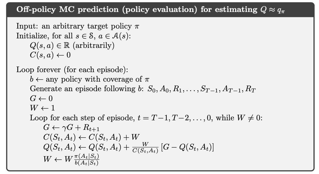
For derivation look here.

5.7 Off-policy MC Control

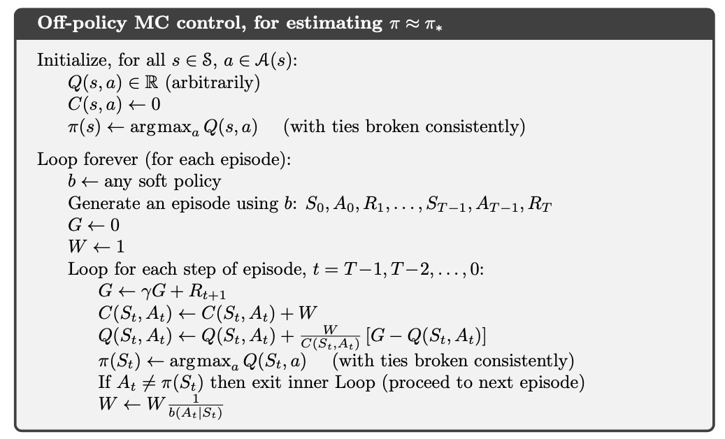
The behaviour policy can be anything, but in order to assure convergence of \(\pi\) to the optimal policy an infinite number of returns must be obtained for all posisble state-action pairs, which is achieved using \(\epsilon-soft\) policy. A potential problem is that tthis method only learns from the tails of episodes, when all the remaining actions in the episode are greedy. If non-greedy actions are common, then learning will be slow, particularly states appearing in the early poritions of long episodes. Potentially this could greatly slow learning.