Chapter 6: Temporal Difference Learning
Learning from Experiences minus the Complete Rollout
INDEX
These are just my notes of the book Reinforcement Learning: An Introduction, all the credit for book goes to the authors and other contributors. My solutions to the exercises are on this page. Addtional concise notes for this chapter here. There is also a Deepmind's Youtube Lecture and slides for model free value extimation and model free control. Some other slides.
We do not know what the rules of the game are; all we are allowed to do is watch the playing. Of course if we are allowed to watch long enough we may catch on a few rules. - Richard Feynman
6.1 TD Prediction
From Monte-Carlo we know that value update formula is given as \[V(S_t) \leftarrow V(S_t) + \alpha(G_t - V(S_t))\] however one limitation is that it depends upon the complete roll out of any episode, we can however calculate the estimated return for any state as \(G_t = R_{t+1} + \gamma V(S_{t+1})\) and replace it in the equation to get \[V(S_t) \leftarrow V(S_t) + \alpha(R_t + \gamma V(S_{t+1}) - V(S_t))\] We call \(R_t + \gamma V(S_{t+1})\) TD target and \(\delta_t = R_t + \gamma V(S_{t+1}) - V(S_t)\) the TD error. Since this is just one step look-ahead it is called TD(\(0\)) which is a special case of n-step TD and TD(\(\lambda\)). We use the idea of bootstrapping, that we start off with a guess make a move and based on the returns update our original guess.

Tabular TD(\(0\)) for estimating \(v_\pi\)
\[v_\pi(s) = \mathbb{E}[G_t|S_t = s]\] \[v_\pi(s) = \mathbb{E}[R_{t+1} + \gamma v_\pi(S_{t+1})|S_t = s]\] We can say that the upper equation is what the MC use as estimates and lower is what DP use as estimates for any state. Notice that the TD error \(\delta_t\) is the error made in estimate at that time. Because the TD error depends on the next state and next reward, it is not available until one time step later. We can calculate the Monte Carlo error as sum of TD errors from that point. \[ G_t - V(S_t) = R_{t+1} + \gamma G_{t+1} - V(S_t) + \\ \gamma V(S_{t+1}) -\gamma V(S_{t+1}) \] \[= \delta_t + \gamma (G_{t+1} - V(S_{t+1}))\] we can now continue to substitute the values and see the expansion as \[ = \delta_t + \gamma\delta_{t+1} + \gamma^2\delta_{t+2} + ... \\ \gamma^{T-t-1}\delta_{T-1} + \gamma^{T-t}(G_T -V(S_T)) \] \[ = \delta_t + \gamma\delta_{t+1} + \gamma^2\delta_{t+2} + ... \\ \gamma^{T-t-1}\delta_{T-1} + \gamma^{T-t}(0 - 0) \] \[\delta^{TD}_t = \sum_{k=t}^{T-t}\gamma^{k-t}\delta_k\] This identity is not exact if the \(V\) changes during the episode eg. an update, but if the step size is small it may still hold approximately. When \(V\) updates following changes will have to be made.
Example 6.1: Driving Home The aim is to predict the Total Time required to get home, which will be the sum of columns one and columns two.
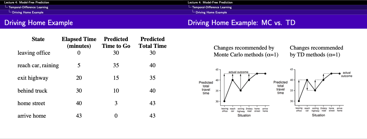
If our aim is to predict total time then how MC would compare against TD
Must you wait until you get home to before increasing your estimate for initial state? According to Monte Carlo approahc you must, because you don't yet know the true return. According to TD approach, on the other hand, you would learn immidiately, shifting your intial estimate from 30 minutes towards 50. In fact, each estimate would be shifted toward the estimate that immidiately follows it.
6.2 Advantage of TD Prediction
There are clear advantages like, TD can learn without a final outcome or in non-episodic settings (continuous). Another advantage is that TD does not require the complete episode it to end, it just has to look one step ahead. For any fixed policy \(\pi\), TD(\(0\)) has been shown to converge to \(v_\pi\), though most convergence proof apply on table-based case of the algoithm some also apply to the general linear function approximation.
So if both the TD and MC are proven to converge then the question are which get there first, which learns faster, which makes hte most efficient use of limited data. This is currently an open question as we do not even know how to mathematically prove the question. In practice however constant-\(\alpha\) method have been found to converge faster on stochastic tasks.
The return \(G_t = R_{t+1} + \gamma R_{t+2} + ... + \gamma^{T-1}R_{T}\) is the unbiased estimate of \(v_\pi(S_t)\) same as the true TD target \(R_{t+1} + \gamma v_\pi(S_{t+1})\) (as if someone has already given us the true value function \(v_\pi\)). However TD target \(R_{t+1} + \gamma V(S_{t+1})\) is a biased estimate of \(v_\pi(S_t)\), because the estimate \(V(S_{t+1})\) can be wildly wrong.
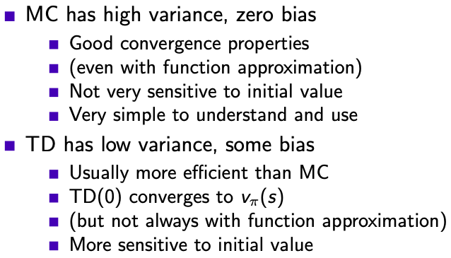
MC vs. TD
6.3 Optimality of TD(\(0\))
If we have to approximate the value function V at we have just a few episodes or a few samples, we can pass over all the values and calculate the sum of all increments. We then apply this sum of all increments to change the value function \(V\) unlike applying for each sample/episode. This is called batch updating because updates are made only after processing each complete batch of training data.
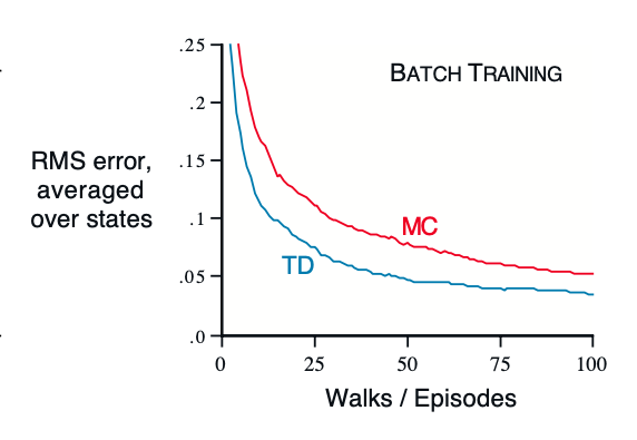
Performance of TD(\(0\)) and constant-\(\alpha\) MC under batch training on random walk task
Example 6.3 Under the batch training, the constant-\(\alpha\) MC converges to \(V(s)\), that are sample averages of actual returns after visitin each state \(s\). These are optimal estimates in the sense that they minimize the MSE, still TD method was able to outperform and get better MSE scores. The question is why is that. Figure above.
Example 6.4 In this example we are given a simple process and we have to estimate the value of the states \(V(A)\) and \(V(B)\). By using MC method we get values \(V(B) = 0.75\) and \(V(A) = 0\), whereas if we us TD we get \(V(B) = 0.75\) and \(V(A) = 0.75\). And both are legitimate values, then why do we get this difference in values. That is because MC gives best fit to observed state \[\sum_{k=1}^K\sum_{t-1}^{T_K}\big(g_t^k - V(S_t^k)\big)^2\] where as the TD\((0)\) converges to solution of MDP that best explains the data. So it first fits the transitions and then calculates the value for that from the rewards. In general the maximum likelyhood estimate of a parameter is the parameter-value whose probability of generating data is maximum. Given this MDP we can compute the estimate of the value function that would be exactly correct if the model was exactly correct. This is called certainity-equivalenge estimate because it is equivalent to to assuming that the estimate of underlying process what known with certainity rather than being approximated.
This explains why TD\((0)\) methods converge faster nad more quickly than MC methods. In batch form, TD\((0)\) is faster than MC becuase it computes the true certainity-equivalence estimate. Finally it is interesting to note that if \(n = |S|\) then calculating MLE requires \(n^2\) memory and \(n^3\) computational steps if done conventionally. In these terms it is striking that TD methods can approximate the same solution using memory no more than \(n\) and repeated computations over the training set.
6.4 SARSA; On-policy TD-Control
Now we have reached the most popular learning algorithm, probably in all of RL that is Sarsa. The idea of sarsa is simple, you start with a state, action pair (\(S,A\)), you sample the environment and get reward \(R\) and end up in state \(S'\) and sample our policy to take the action \(A'\) i.e. \(S,A,R,S',A'\). Here we still follow the pattern of Generalised policy iteration and action-value funcion \(q_\pi(s,a)\) instead of value-function \(v(s)\). This can be done essentially the same TD method described above for learning \(v_\pi\) applied to \(q_\pi\)

Transition diagram
We consider the transitions and get equation as \[ Q(S_t, A_t) \leftarrow Q(S_t, A_t) + \\ \alpha [R_{t+1} + \gamma Q(S_{t+1}, A_{t+1}) - Q(S_t, A_t)] \] This update is done for each non-terminal state \(S_t\) for terminal state \(S_{t+1}\) we define \(Q(S_{t+1}, A_{t+1}) = 0\). The convergence properties of the Sarsa depend on the nature of policy's dependence on \(Q\), eg. one could use \(\epsilon\)-greedy or \(\epsilon\)-soft policies. Sarsa converges to probability 1 to an optimal policy and action-value function as long as all the state-actions have been visited \(\infty\) times.

Sarsa (On-policy TD Control) for estimating \(Q \approx q_*\)
6.5 Q-Learning; Off-policy TD-Control
This is single handedly the first Deep-RL algorithm anyone tries to imeplement, thanks to Deepmind. The idea was first defined by Watkins, 1989 in his Ph.D thesis titles Learning from Delayed Rewards. It is defined as follows: \[ Q(S_t, A_t) \leftarrow Q(S_t, A_t) + \\ \alpha [R_{t+1} + \gamma \max_aQ(S_{t+1}, A_{t+1}) - Q(S_t, A_t)] \] And the algorithm is given as follows

Q-Learning (Off-policy TD Control) for estimating \(\pi \approx \pi_*\)
Example 6.6 Cliff Walking In this example we find that Q-learning learns the optimal path of walking just next to the cliff while Sarsa learns the safest policy of walking as far from the cliff as possible. For Q-learning though this means it occasionally falls off the cliff because of \(\epsilon\)-greedy policy. Of course if the \(\epsilon\) were to be gradually reduced, then both methods would asymptotically converge to the optimal policy.

right: cliff environment setup | left: rewards by the two algorithms
6.6 Expected Sarsa
Consider that we converted in \(G_t = \mathbb{E}_\pi[Q(S_{t+1}, A_{t+1}) | S_{t+1}]\) to proper expectations as \(G_t = \sum_a\pi(a|S_{t+1})Q(S_{t+1},a)\). We call this expected Sarsa, and since we remove the samlping of action given the probability we can eliminate the variance and this should result in better performance and that indeed is what we see.
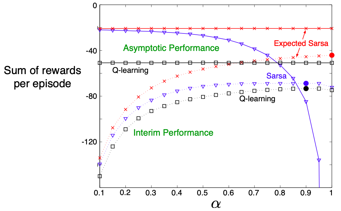
Interim (dashed) and Asymptotic (solid) are calculated by getting averages from first 10 and 50,000 runs. Solid Circle shows the best performance for interim performance
It can also learn over a wide variety of step-sizes, it can safely set \(\alpha=1.0\) without suffering any degradation of asymptotic performance. In the cliff walking results Expected Sarsa was used on-policy, but in general it might use a policy different from the one learning and so it becomes off-policy in that way, which is basically Q-Learning.
6.7 Maximisation Bias and Double Learning
In these algorithms, a maximum over estimates values is used implicitly as an estimate of the maximum value, which can lead to a significant positive bias. Consider a state \(s\) where many actions \(a\) whose true values \(q(s,a) = 0\) but the estimated values \(Q(s,a) \neq 0\), some are above and some are below zero. The maximum of true values is zero but the maximum of estimates is positive, maximisation bias. Consider the simple MDP below, the ideal solution is to never take left since the distribution is very likely to return negative rewards. But Q-learning will over estimate the value of B and chose that.
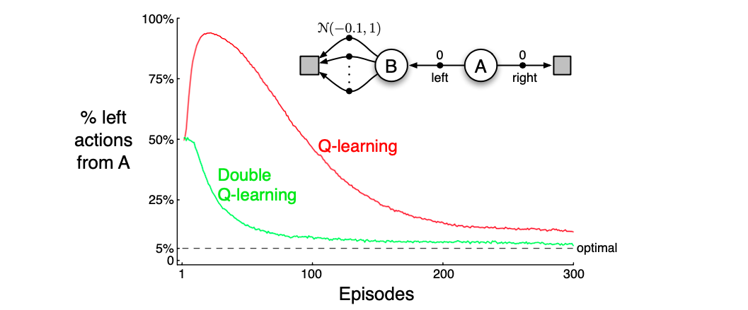
Q vs. Double-Q for the given MDP
So how to we handle this maximisation bias, one way is to introduce two q-values. One q-value \(Q_1\) to determine the maximising action \(A^* = argmax_a Q_1(a) \) and another \(Q_2\), to provide the estimate of its value \(Q_2(A^*) = Q_2(argmax_a Q_1(a))\). Both \(Q_1(a)\) and \(Q_2(a)\) are estimates of the true value \(q(a)\) for all \(a \in A\). The estimate is unbiased in the sense that \(\mathbb{E}[Q_2(A^*)] = q(A^*)\), and we can reverse the roll and say \(Q_1(A^*) = Q_1(argmax_a Q_2(a))\). The update then becomes \[ Q_1(S_t, A_t) \leftarrow Q_1(S_t, A_t) + \\ \alpha [R_{t+1} + \gamma Q_2(S_{t+1}, argmax_a Q_1(S_{t+1}, A_{t+1})) \\ - Q_1(S_t, A_t)] \] This is the idea of double learning, and the algorithm is given below.
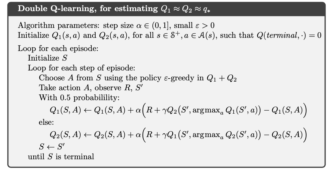
Double Q-learning, for estimating \(Q_1 \approx Q_2 \approx q_*\)
6.8 Games, Afterstates, and Other Special Cases
In our algorithms we depend on the value of the next state, so when we reach the next state (afterstate) the values should be applied on all the state-actions that make it reach there. As in the diagram below we see that two state-action pairs make it reach the same "afterposition". Afterstates arise in many tasks, not jsut games. For example, in queuing tasks there are actions such as assigning customers to servers, rejecting customers, or discarding information. In such cases the action are in fact defined in tersm of their immediate effects, which are completely known.
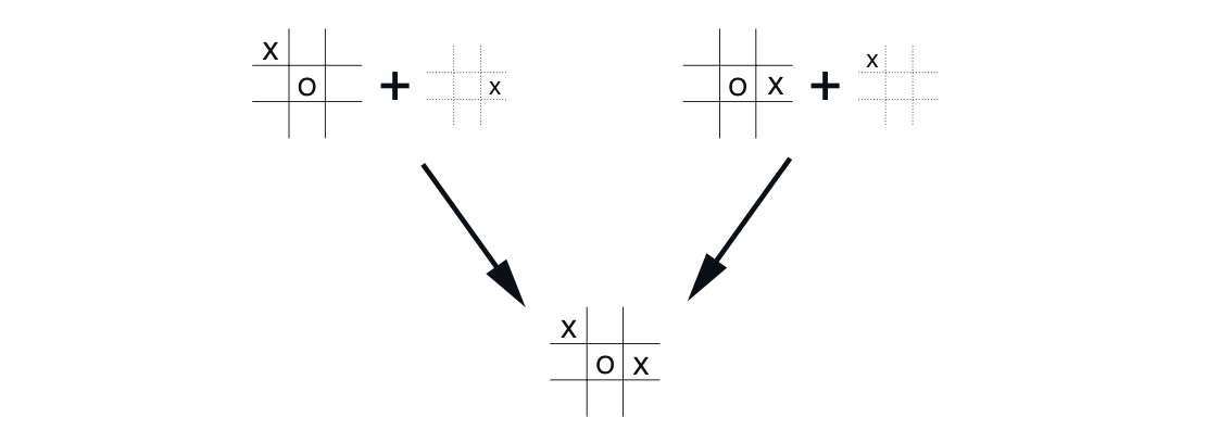
two state-action pairs make board reach the same "afterposition"