Chess Engine - (Part 1.5)
On scaling laws for Language Models
This is first in a series of blogs covering this project. TL;DR see this Github repo. Also for all you who do not understand the Indian number system just read this wiki. This is a follow up to my previous work where I train a language model on \(25Cr\) or \(225.1Mn\) moves and pose some questions.
If you have any freelancing work, contact me on my LinkedIn.
Initially this was going to be do and done kind of project but now it seems like this is going to take a while and if I am lucky I might just get a paper out of it. There are so many shitty papers out there that you can't believe something so meaningless can get a paper out. But anyways, it's them and we gotta do our योग. This blog is mostly a paper discussion and will be a quick one.
📶 What are power laws
It used to be when compute was low that simply adding more layers to a network used to work. But this paradigm changed with very large model (GPT-2, BERT, T5, etc.) and with the investment in these softwares it became important to know how these model actually scale, what matters and what not. So OpenAI did a research and answered those questions based on Power Law. So we start our discussion with what is a powerlaw.
Powerlaws are mathematical relationship where changing one value causes a proportional change in the outcome or power law is a function \(f(x)\) where the value \(y\) is proportional to some value of \(x\). Eg. doubling the length makes area \(4\) times and volume \(8\) times. So we can give it a form \(A(x) \propto x^k\) where \(k = 2\) and when considering volume \(k = 3\). Such functions have three properties:
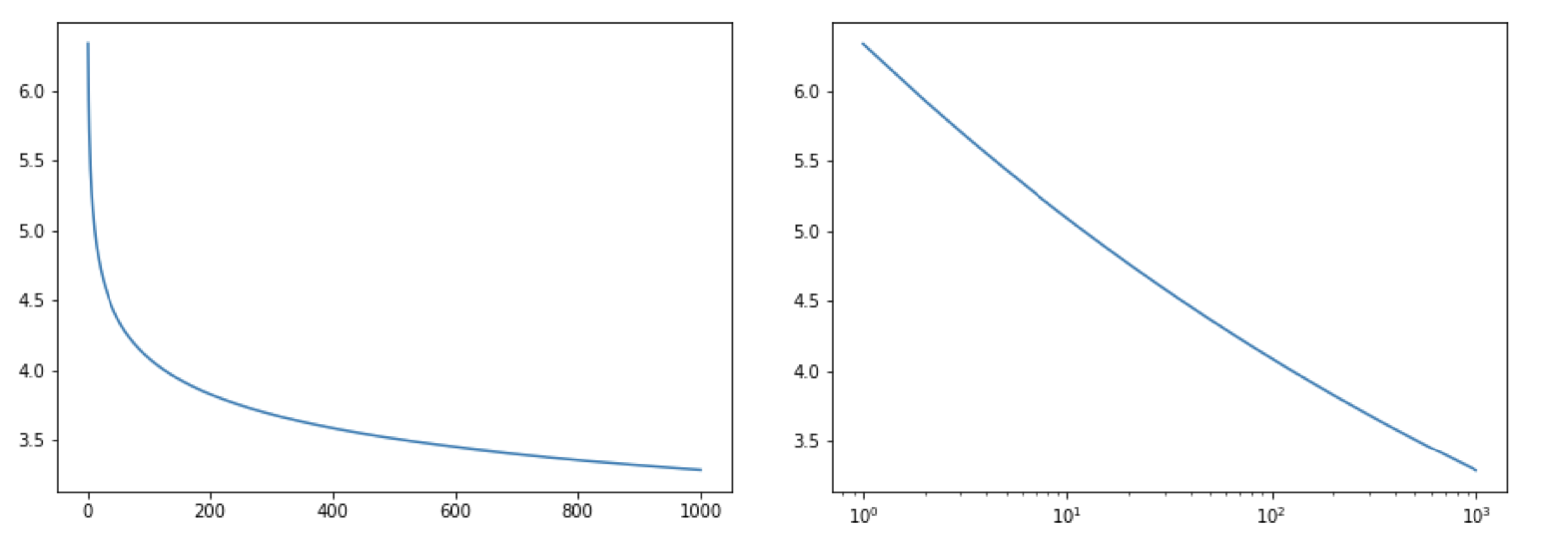
(Left) you have normal power law distribution and (Right) shows that scaling x-axis to log gives a linear graph. Which helps when working exponentially increasing/decreasing values. \(y = f(x) = 5.6 x^{-0.095} \forall x \in [0,1000) \)
📶 How to make network bigger (PROPERLY)
The paper we are dealing with today is called "Scaling Laws for Neural Language Models" (ArXiv) by OpenAI. With the knowledge of the power laws it becomes easier to predict things at scale and this is helpful as neural networks grow exponentially in size. But we start with defining the nomenclature:
Parameter counts and compute (forward pass) estimates for a Transformer model. Sub-leading terms such as nonlinearities, biases, and layer normalization are omitted.
What are the lesson learnt, those with images are given below the bullet points:
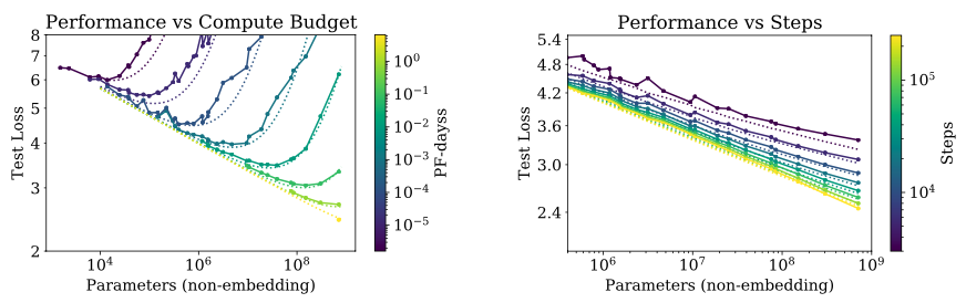
(left) It means that for a given compute size there is an optimal model size (where the loss is lowest, on the line) and for the same amout of compute both the larger and the smaller models can give the same results (test loss). Thus we should find the optimal model for this compute size. (right) at same steps, larger models give lower loss and on increasing the steps there is decrease in loss for the same model.
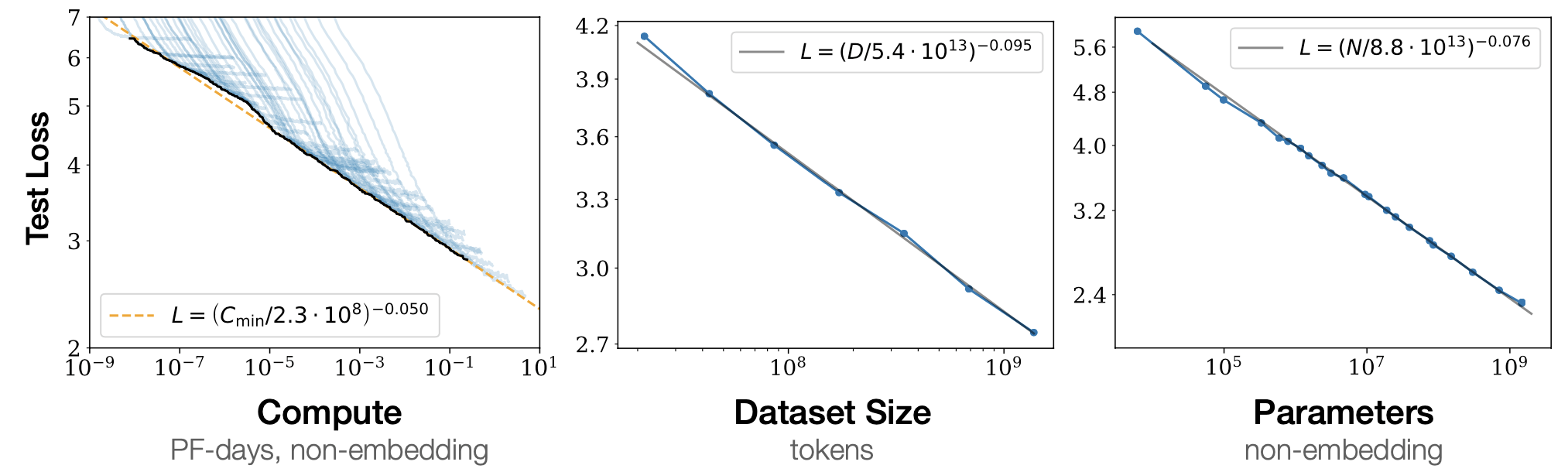
This has to be the best representation of results. What this shows is that for each variable shown, if the other two are optimal then the test loss is very predictable and follows smooth curves. Thus in order to train an efficient model we need to grow all three in tandem. This is the engineering challenge!
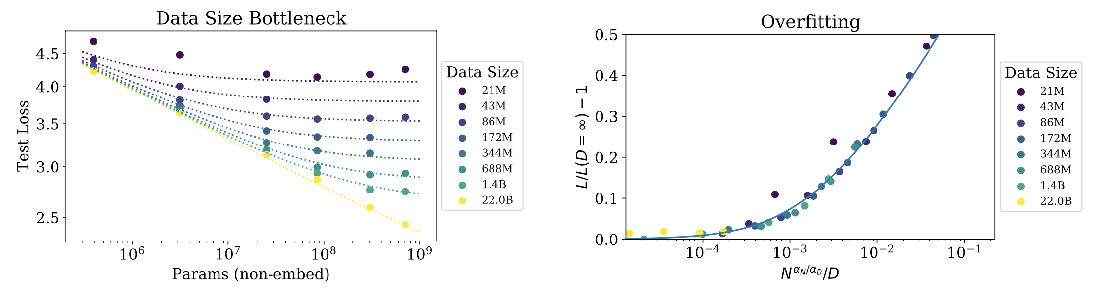
This is another important graph. On the right you see that datasize can also become a bottleneck (😓 this sounds familiar), ie. when you have a small dataset even larger models can suffer same loss. When this happens no amount of compute or model size increase can help you and you start to move away from efficient frontier. On the right is the For reference: \(L(N,D) = \Big( (\frac{N_C}{N})^{\frac{\alpha_N}{\alpha_D}} + \frac{D_C}{D} \Big)^{\alpha_D}\) and on right, X-axis is \(N^{0.737}/D\).
So what is the problem?
Kolmogorov defined the complexity of a string \(\text{x}\) as the length of its shortest description \(\text{p}\) on a universal Turing machine \(\text{U(K(x))} = \min\{\text{l(p):U(p)=x}\}\), .