Chapter 4: Dynamic Programming
Solving Finite MDP
INDEX
These are just my notes of the book Reinforcement Learning: An Introduction, all the credit for book goes to the authors and other contributors. My solutions to the exercises are on this page. Addtional concise notes for this chapter here. There is also a Deepmind's Youtube Lecture and slides. Some other slides.
We do not know what the rules of the game are; all we are allowed to do is watch the playing. Of course if we are allowed to watch long enough we may catch on a few rules. - Richard Feynman
Introduction
Dynamic Programming means optimising a "program" (which we call policy) over a temporal problem. It is a method used for solving complex problems by breaking them down into simpler smaller sub problems. Following are the requirements for DP:
Dynamic programming is used in other places as well scheduling algorithms, sequence alignment, shortest path, graphical problems, bioinformatics (lattice models), etc. Dynamic programming assumes full knowledge of MDP. They are used for two different things:
4.1 Policy Evaluation (Prediction)
Although DP ideas can be applied to problems with continuous state and action spaces, axact solutions are only possible in special cases. Recall from Chapter 3 we get value of state from following function. \[v_\pi(s) = \mathbb{E}_\pi \left[ G_t | S_t = s \right] \] \[= \mathbb{E}_\pi \left[R_{t+1} + \gamma G_{t+1} | S_t = s\right] \] \[= \mathbb{E}_\pi \left[R_{t+1} + \gamma v_\pi(S_{t+1}) | S_t = s\right] \] \[= \sum_a \pi (a|s) \sum_{s',r} p(s',r|s, a) \left[r + \gamma v_\pi(s')\right] \tag{1} \] Consider a sequence of approximate value functions \(v_0, v_1, v_2, ...\), each mapping \(S^+\) to \(\mathbb{R}\). The initial approximation, \(v_0\), is chosen arbitrarily (except that the terminal, if any, must be given value \(0\)), and each succesive approxiamtion is obtained by using the Bellman equtaion for \(v_\pi (0)\) as an update. \[v_{k+1} = \sum_a \pi (a|s) \sum_{s',r} p(s',r|s, a) \left[r + \gamma v_k(s')\right] \tag{2}\] Indeed it can be shown in general to converge to \(v_\pi\) as \(k \rightarrow \infty\) under the same conditions that guarantees the existence of \(v_\pi\). This algorithm is called interative policy evaluation. All the updates done in DP algorithms are called expected updates because they are based on an expectation over all possible next states rather than on the sample next state. We think of the updates being done in a sweep through the state space (instead of using the two array method).
4.2 Policy Improvement
We know how good it is to follow the current policy \(\pi\) from \(s\) i.e. \(v_\pi(s)\), but would it be for better or worse to change to the new policy? One way to answer this is to consider selecting \(a\) in \(s\) and thereafter following the existing policy \(\pi\). \[q_\pi(s,a) = \sum_{s',r}p(s',r|s,a) \left[r + \gamma v_\pi(s') \right]\] If this is greater than the value \(v_\pi(s)\), we can assume that taking action \(a\) everytime \(s\) is encounters, would be a better policy. That this is true is special case called the policy improvement theorem. Let \(\pi\) and \(\pi'\) be any pair of deterministic policies such that \(\forall s \in S\) \[v_\pi(s) \leq q_\pi(s, \pi'(s) \tag{1}\] \[\leq \mathbb{E}\left[R_{t+1} + \gamma v_\pi(S_{t+1}) | S_t = s, A_t = \pi'(s)\right]\] \[\leq \mathbb{E}_\pi'\left[R_{t+1} + \gamma v_\pi(S_{t+1}) | S_t = s\right]\] \[\leq \mathbb{E}_\pi'\left[R_{t+1} + \gamma q_\pi(S_{t+1}, \pi'(S_{t+1})) | S_t = s\right]\] \[\leq \mathbb{E}_\pi'\left[R_{t+1} + \gamma R_{t+2} + \gamma^2 v_\pi(S_{t+2}) | S_t = s\right]\] \[\leq \mathbb{E}_\pi'\left[R_{t+1} + \gamma R_{t+2} + \gamma^2 R_{t+3} + ... | S_t = s\right]\] \[\leq \mathbb{E}_\pi'\left[R_{t+1} + \gamma v_\pi(S_{t+1}) | S_t = s\right]\] \[v_\pi(s) \leq v_\pi'(s) \tag{2}\] That is if there is strict inequality of \((1)\) then there will be strict inequality of \((2)\). Thus is \(q_\pi(s, a) > v_\pi(s); a = \pi'(s)\) then the changed policy is indeed a better than \(\pi\). Thus at each step we select the best possible \(q_\pi(s,a)\) at each step, basically greedy policy. \[\pi'(s) = \max_a q_\pi(s,a) = \max_a \sum_{s',r}p(s',r|s,a)\left[r + \gamma v_\pi(s')\right] \tag{3}\] By construction, the greedy policy meets the conditions of policy improvement theorem \((1)\), so we know that is as good as, or better than the original policy. Suppose the new policy \(v_{\pi'} = v_\pi\) then it follows that \(\forall s \in S\), \((3)\) is true. But this is same as Bellman optimality equation and therefore, \(v_{\pi'}\) must be \(v_*\) and both \(\pi\) and \(\pi'\) must be optimal policy. Now there is a simple way to improve the policy, firstly Evaluate the policy \(\pi\) as in \(v_\pi\) and secondly, improve the policy \(\pi\) by acting greedily w.r.t. \(v_\pi\)
4.3 Policy Iteration
The idea of policy improvement is very simple as follows: if any policy \(\pi\) has been improved using \(v_\pi\) to yeild a better policy \(\pi'\), we can then compute \v_{\pi'}\) and improve it again to yeild an even better \(\pi^{''}\). We can thus obtain a sequence of monotonically improving policies and value functions like:
\(E\) is evaluation and \(I\) is improvement
Example 4.2: Jack's Car Rental This is a detailed question where we have to calculate how many cars need to be transferred in either of two locations and cost of it, given that Jack gets profit for renting out the cars. This question can be broken down as follows, state is that any location can have a maximum of 20 cars. Actions are to move upto 5 cars overnight, reward is \($10\) for rented car and \(-$2\) for moving a car overnight and transitions are poisson probability distribution.
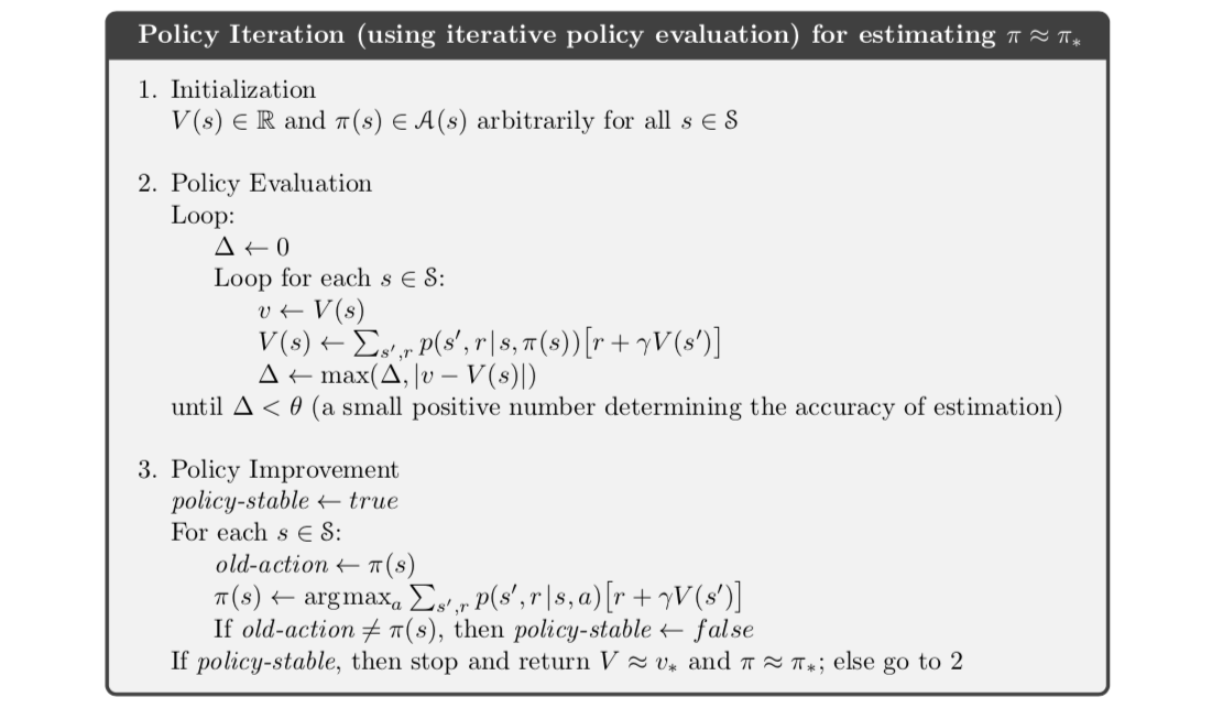
Policy Iteration Algorithm
Can we use something to truncate over value evaluation and stop at some point. We can look at the Bellman error and say how much we want to refine our error, if there is not a lot of difference then we can stop (\(\epsilon\)-convergence). Secondly simply stop after \(k\) iterations of iterative policy evaluation. Extreme case of this would be stop after \(k=1\) iterations and this then becomes value iteration.
4.4 Value Iteration
If policy evaluation is done iteratively, then convergence exactly to \(v_\pi\) occurs only in the limit, should we wait for exact convergence, or can we stop early? In fact, the policy evaluation step id policy iteration can be truncated in several ways without losing guarantees of policy iteration. One important special case is when the policy evaluation is stopped after just one sweep (one update of each state). \[v_{k+1} = \max_a \sum_{s',r}p(s',r|s,a) \left[r + \gamma v_k(s') \right]\] Faster convergence is often achieved by interposing multiple policy evaluation sweeps between each policy improvement.
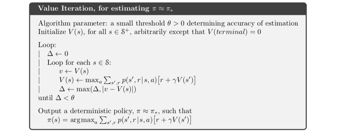
Value Iteration Algorithm
4.5 Asynchronous Dynamic Programming
DP by default is not very fast and there are multiple improvements that can be made to make DP faster. Namely, in-Place, sweeping and real time. I am not going in detail for each and can be understood easily from book, lecture and slides.
4.6 Generalised Policy Iteration
The value function stabilizes only when it is consistent with the current policy, and the policy stabilizes only when it is greedy with respect to the current value function. Thus both the processes stabilize only when a policy has been found which is greedy with respect to its own evaluation functions. This implies that Belmann optimality equation holds adn thus that the policy and value function are optimal. In either case, the two processes together achieve the overall goal of optimality even though neither is attempting to achieve it directly.
Generalised Policy Iteration
Extra: How video's nomenclature is related to book's
In the book equation for value iteration and in lectures it is given as follows: \[v_{k+1} = \max_a \sum_{s',r} p(s',r|s, a) \left[r + \gamma v_k(s')\right]\] \[v_{k+1}(s) = \max_a \left( R_s^a + \gamma \sum_{s'} P_{ss'}^a v_k(s)\right)\] We can derive this in the following manner \[v_{k+1} = \max_a \sum_{s',r} p(s',r|s, a) \left[r + \gamma v_k(s')\right]\] \[= \max_a \left(\sum_{s',r} p(s',r|s, a) r + \gamma \sum_{s',r} p(s',r|s, a) v_k(s') \right)\] Now we can expand \(\sum_{s',r} p(s',r|s, a)\) like \(\sum_{s'} p(s'|s, a) \cdot \left( \sum_r p(r|s,a) \right)\). Thus the above equation becomes as follows \[= \max_a \left(\sum_{s'} p(s'|s, a)\left( \sum_r p(r|s,a) r \right) + \\ \gamma \sum_{r} p(r|s, a)\left( \sum_{s'} p(s'|s,a) v_k(s') \right) \right)\] We can now combine \(\sum_r p(r|s,a) r = R_s^a\) and \(p(s'|s,a) = P_{ss'}^a\), thus we get the equation \[= \max_a \left(\sum_{s'} p(s'|s, a) R_s^a + \gamma \sum_{r} p(r|s, a)\left( \sum_{s'} P_{ss'}^a v_k(s') \right) \right)\] As the inside elements are independent of the outer sum elements they can be brought outside the summation \[= \max_a \left( R_s^a \sum_{s'} p(s'|s, a) + \gamma \left( \sum_{s'} P_{ss'}^a v_k(s') \right) \sum_{r} p(r|s, a) \right)\] Now the value of summations is going to be \(1\) as they are sum of probabilities, we can write the above equation as \[v_{k+1}(s) = \max_a \left( R_s^a + \gamma \sum_{s'} P_{ss'}^a v_k(s')\right)\]