Reading List on Neural Graph Execution
Lets Call this Neural Algorithm Execution (NAE)
With my previous machine learning "algorithms" post I showed a quick hack kind of poisisbility that we can teach the machines algorithms. For verification of that I trained a simple convnet on Conway's game of life cellular automata, which is application of three simple rules. I also have been working on Graph Neural Networks and they seemed very powerful but at the same time weak. While browsing the internet I found this talk on topic "Graph Representation Learning for Algorithmic Reasoning" and so these are the quick notes on the topic. For reference you can use the slides here. This is a reading list kind of thing where I also write the notes on those. TL;DR just want the conclusions
Declaration: These are just my notes on the topic that I am providing on my website. All the credit for the work goes to the respective authors. As far as possible I have tried to provide links to the papers and articles I have used. If I have missed some or you have any suggestions please ping me at bonde.yash97@gmail.com or linkedin or twitter.
INDEX
Why do this when I have algorithms?
This is a good question that if I have already spent some time on making an algorithm then why would I want to add a layer of training nueral network. Neural Networks (+) operate on raw inputs, (+) Generalise on noisy conditions, (+) models reusable across tasks but (-) require big data, (-) unreliable when extrapolating and (-) there is a lack of interpretability.
Classical algorithms on the other hand (+) trivially strongly generalise, (+) compositional (subroutines), (+) guaranteed correctness, (+) interpretable operations but (-) inputs must match spec and (-) not robust to task variations. Is it possible to get the best of both worlds?
Issues with Datasets, Models (Benchmarking GNNs)
Pitfalls of Graph Neural Network Evaluation (Schur et al.)
In this paper authors tell how the current datasets and models are bad metrics to find the optimal models. The comparison was done on 3 major dataset CORA, CiteSeer, PubMed and the main results was that different splits lead to a completely different ranking of models. Our results highlight the fragility of experimental setups that consider only a single train/validation/test split of the data. We also find that, surprisingly, a simple GCN model can outperform the more sophisticated GNN architectures if the same hyperparameter selection and training procedures are used, and the results are averaged over multiple data splits.
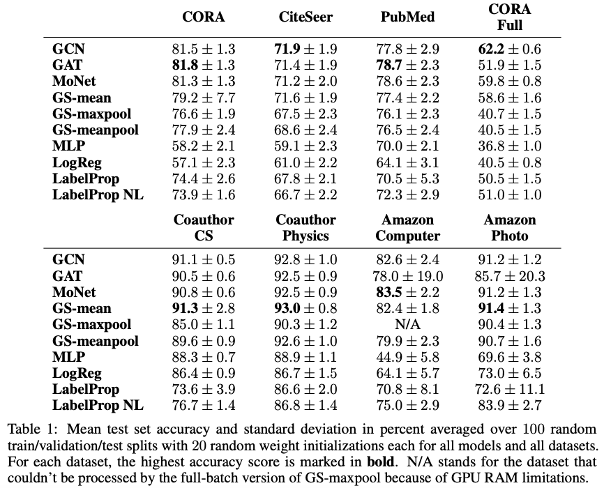
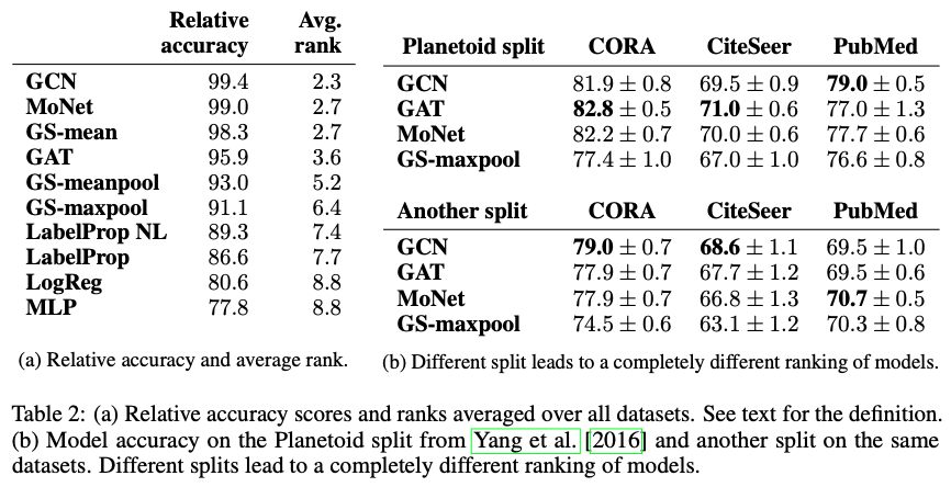
The above two are screenshots from this paper
In addition, we consider four baseline models. Logistic Regression (LogReg) and Multilayer Perceptron (MLP) are attribute-based models that do not consider the graph structure. Label Propagation (LabelProp) and Normalized Laplacian Label Propagation (LabelProp NL), on the other hand, only consider the graph structure and ignore the node attributes.
On Graph Classification Networks, Datasets and Baselines (Luzhnica et al.)
Authors show that despite recent advanced in GNNs the competitive performance is achieved by the simplest of models – structure-blind MLP, single- layer GCN and fixed-weight GCN. For simple baseline two models are considered:
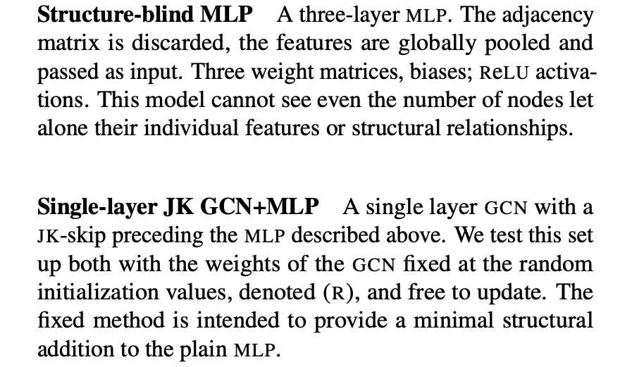
Now going over the benchmark comparisons we see that majority cases the GNN models perform worse to MLP (blue).
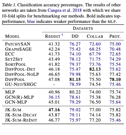
The above two are screenshots from this paper
This brings to question a couple of things, whether the datasets really require the advantages that GNNs provide, as we can see in many cases that is not even true. The other way to see it is whether the implementations of GNNs really allows it to be powerful over basic MLP.
Simplifying Graph Convolutional Networks (Wu et al.)
Paper that shows how reducing the GCN by removing non-linearities and collapsing weight matrices between consecutive layers, then the model corresponds to a fixed low-pass filter followed by a linear classifier. This is a pretty smart paper where they explain how the entire graph layers with regularities between graph removed is nothing but a feature extraction preprocessing layer. More details in the diagram below:
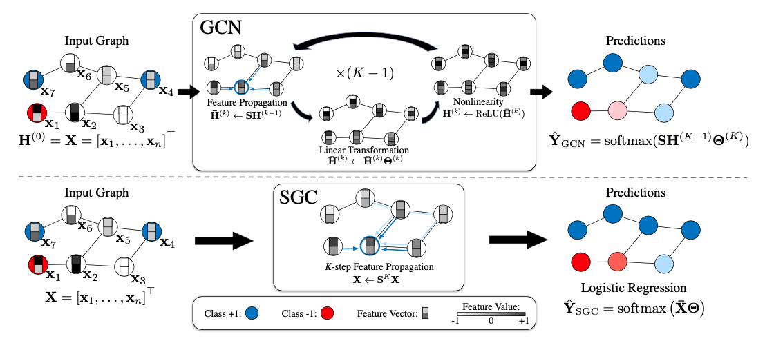
from here
The idea is discussed in Section 2, first they explain the conventional Graph Convolutional Network (GCN). Feature propogation is what separates GCN from MLP, at the beggining of each layers is the features \(h_i\) for each node \(v_i\) which are averaged in the local neighbourhood: \[h_i^{(k)} \leftarrow \frac{1}{d_i + 1}h_i^{(k+1)} + \sum_{j=1}^{n}\frac{a_{ij}}{\sqrt{(d_i + 1)(d_j + 1)}}h_j^{(k-1)}\] Let \(S\) denote the normalised adjacency matrix with self-added loops \(S = D^{-\frac{1}{2}}\overline{A}D^{-\frac{1}{2}}\) where \(\overline{A} = A + I\), \(A\) is adjacency matrix and \(D\) is degree matrix. So we can reduce the above formula \[H^{(k)} \leftarrow SH^{(k-1)}\] Now each layer will also have a learned matrix \(\Theta\) and so we can write propogation for each layer happens as \[H^{(k)} \leftarrow ReLU(SH^{(k-1)}, \Theta^{(k)})\] and finally we get to the predictions using softmax as \[Y_{GCN} = softmax(SH^{(k-1)}, \Theta^{(k)})\]
We see that with increasing depth in MLP it becomes more feature heirarchical as a layers features depend on the features from its previous layers. In GCN the equivalence is that k-layers mean that information from k-hops away is aggregated. Based on this idea authors perform linearisation in which all the non-linearities in layers are removed, so we are left with chain of normalised adjacency matrices and learned weight matrices. So output of the network becomes \[Y = softmax(S ... S X \Theta^{(1)} ... \Theta^{(K)})\] We can compress them as \(S^K = S ... S\) and \(\Theta = \Theta^{(1)} ... \Theta^{(K)}\) and so we get the output distribution as \[Y_{SGC} = softmax(S^K X \Theta)\] SGC distinguishes between feature extraction and classifier, SGC consists of a fixed (i.e., parameter-free) feature extraction/smoothing component \(\overline{X} = S^KX\) followed by a logistic regression classifier \(Y = softmax(\overline{X} \Theta)\). So we can think of it like performing preprocessing for k-hops and then performing LR.
The paper then has some giant math spaghetti, I am not going to get into where they mathematically prove that under such setup the preprocessing layers behave as a low-pass filter.

from here
Ultimately, the strong performance of SGC sheds light onto GCNs. It is likely that the expressive power of GCNs originates primarily from the repeated graph propagation (which SGC preserves) rather than the nonlinear feature extraction (which it doesn’t.)
Summarising This section
Popular GNN benchmark datasets often unreliable and the complexity not very high. Training the networks on algorithms might prove to be favourable as we can generate infinite data, perform complex data manipulation and we get that a very clear hierarchy of models emerge (discussed later). Since we use a generating function we do not have noise in the data generated and credit assignment becomes easier.

from here
We can also use this on NP-hard problem such as travelling salesman problem as done in An Efficient Graph Convolutional Network Technique for the Travelling Salesman Problem (Joshi et al.), look at the diagram above. you can see that
From Generalisation point (Strong Generalisation)
Algorithms are not simple data mapping (input-output mapping) but instead the network must learn the underlying manipulations / individual operations. Imitating individual operations enables strong generalisation, consider how humans devise algorithms by hand and scales to much larger graph sizes. This grounds the GNN in the underlying algorithmic reasoning it learns more than just mapping but learns the manipulations.
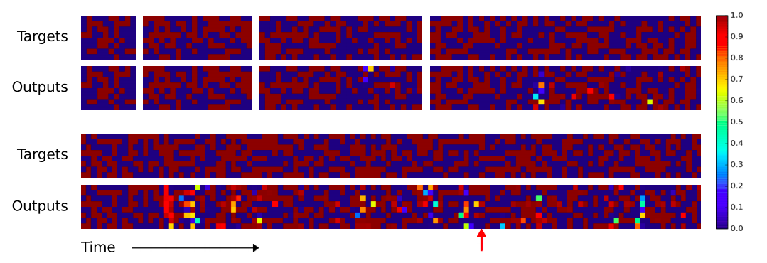
Neural Turing Machine (NTM) on copy task, from here
The two diagrams show different kinds of generalisation. In the above digram we see that when trained on sequence of a particular length when scaling up the copy on longer sequences it fails. Where as in the bottom we see different kind of generalisation, NTM though not trained as composable shows better generalisation on repeat copy task.
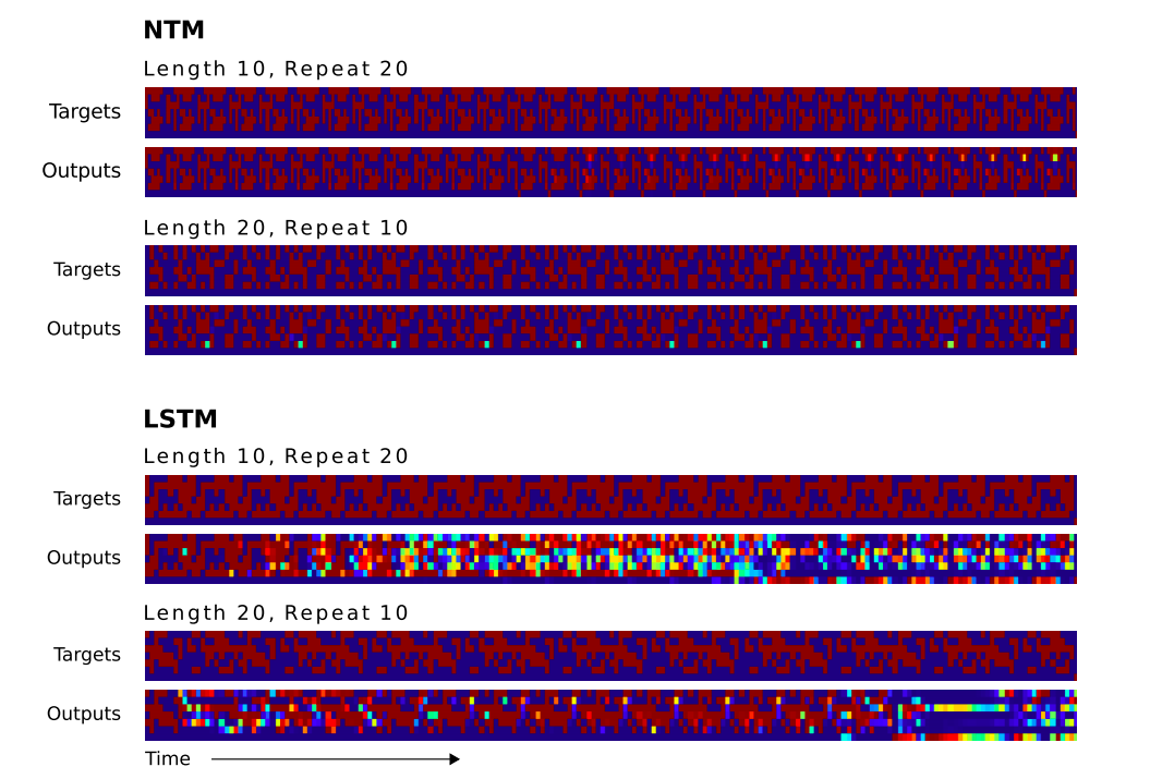
NTM vs. LSTM on repeat-copy task, from here
Later we will see how generalisation can be achieved on NAE and use that to achieve 100% on much different evaluation cases.
Reusing Subroutines (Multitask Learning)
Many algorithms share many parts and vary very little. For comparison compare the Prim's Algorithm and Dijkstra's algorithm. Both of them are used to find the shortest path between two points one using a Minimum Spanning Tree and other using shortest node path. Infact even the algorithms look very similar (share the sub-routines).

from here
Learning representations of manipulations we can then reuse the subroutines that are so massively shared (eg. length of maximum spannign tree and Djikstra's algorithm). Representations and positively reinforce one another and we can get the meta-representation of the algorithms. And also because we can then see the sharing of subroutines we can then have clearly defined task-relations. Output of easier algorithm can be used as input for a harder one, eg. if an alogrithm can learn the breadth first search on unweighted graph (basically shortest-path) we can then use it for weighted graph (which is what Bellman Ford Algorithm is).
Problem solving in hierarchy of control (Discovering Algorithms)
We now see how using NAE allows us to improve and make better algorithms, we can inspect intermediate outputs of an algorithm can decode its behaviour, to understand its behaviour. It gives us opportunity for deriving novel algorithms eg. spanning trees or optimising GPU/TPU performace afterall they too are just computation graphs. SuperProgrammer: An interesting way to look at would be like the perfect problem solver. GNN can perform soft subroutine reuse from polynomial-time algorithms and once it has an arsenal of these it can use those to solve any problem (think competitive programming).

Looking at NAE from conventional programming paradigm, these are the 3 papers discussed below
The idea is to breakdown the execution into three levels, similar to how the conventional programming is broken down. The higher up you go you get more abstract tasks and things that reason at a much higher level. And the lower you go, you get closer to metal more basic operations. In the following subsections I discuss all the three papers, What can Neural Networks Reason About? (Xu et al.),
What can Neural Networks Reason About? (Xu et al.)
This is an interesting paper/idea that sits at the top of the hierarachy of abstractive task and segements the idea in the 4 types: Summary Statistics, Relational Argmax, Dynamic Programming and NP-hard problem (Is there a subset that sums to 0?).

Different types of problems with different logic required
There are four main algorithms that the paper talks about. First is the simple MLP which works well when you have a single-object universe but fails when we have multiple objects. Secondly we have Deep Sets, which consider reasoning on an unordered set, to induce this permutation invariance authors use two MLPs that look like this \[y = MLP_2\big( \sum_{s \in S} MLP_1(X_s) \big)\] And the third are the GNNs whose structure can be given as follows: \[h_s^{(k)} = \sum_{t\in S} MLP_1^{(k)}(h_s^{(k-1)}, h_s^{(k-1)})\] \[h_S = MLP_2 \big( \sum_{s\in S} h_s^{(K)} \big) \] where \(h_s^{(0)} = X_s\). The final algorithm is the NES (Neural Exhaustive Search), given a universe, NES enumerates all subsets of objects and passes each subset through an LSTM followed by a MLP. The results are aggregated with a max-pooling layer and MLP \[ MLP_2 (\max_{\tau \subseteq S} MLP_1 \circ \\ LSTM (X_1, ..., X_{|\tau|}: X_1, ..., X_{|\tau|} \in \tau )) \]

What the framework shows
What the paper showed is that GNNs that are very similar to the existing algorithms perform better to than any abstract method. Thus in order to create better models we must look for architectures that suit an existing algorithms. For reference in the tasks
- Summary Statistics: Since the idea is the to get the aggregation of information from the available modalities. This can be done using deep sets as they are permutation invariant, as shown in the results below.
- Relational Argmax: This is the case where we need relation between multiple objects and as we can see that Deep Sets would not work in this setting as we need propogation of information across the objects but GNNs with even one layer is able to extract the correct information. This is also reflected in the results below.
- Dynamic Programming: In this task there are several rounds of propogation is required and so we can see that the GNNs with more layers are better at extracting the information
- NP-Hard Problem: These are the problems that require a more deeper logic than just the propogation and thus even Deep GNNs perform poorly, while a simple logic works on this.

The above three images are from this paper
Rest of the paper involves massive amounts of mathematics, theorems proves claims etc. Most of the interesting theory on the work is in Section 4. In particular, the answer what tasks a neural network can learn to reason about is done by studying the generalization ability of learning the underlying reasoning processes for a task. And we find that GNNs are good when it comes to tasks that require dynamic programming kind of setup. Paper also introduces algorithmic alignment, neural networks that can learn other reasoning paradigms beyond dynamic programming.
Neural Execution of Graph Algorithms (Veličković et al.)
Unlike the above paper this one stands lower in hierarchy and deals with the stomic steps in the algorithm. The idea is that many classical algorithms share related subroutines: for example, shortest path computation (via the Bellman-Ford algorithm) and breadth-first search both must enumerate sets of edges adjacent to a particular node. Authors show that by learning several algorithms simultaneously and providing a supervision signal, their neural network is able to demonstrate positive knowledge transfer between learning different algorithms.
The basic idea is that along with a continual propogation of node values at each layer we also keep a latent vector for each node at each layer as clear in the diagram below. The architecture is a encoder-processor-decoder architecture. We start with the latent vector \(h_i^{(0)} = 0\) and the encoded inputs \[ z_i^{(t)} = f_A(x_i^{(t)}, h_i^{(t)})\] where \(f_A\) is the encoder network. The set of all input encoded vectors \(Z^{(t)} = \{ z_i^{t} \}_{v \in V} \) and edge features \(E^{(t)} = \{ e_i^t \}_{e \in E}\) are fed to processor network \(P\) to get latent node features \[ H^{(t)} = P(Z^{(t)}, E^{(t)} ) \] The node and algorithm specific outputs are then calculated by the decoder-network, \(g_A\) \[y_i^{(t)} = g_A(z_i^{(t)}, h_i^{(t)})\] Note that the processor also requires a termination network which tells the probability of termination after applying logistic sigmoid activation \(\rho\) \[ \tau^{(t)} = \rho( T_A(H^{(t)}, \overline{H^{(t)})} ) \] where \(\overline{H^{(t)}} = \frac{1}{|V|}\sum_{i \in V} H^{(t)}\) is the mean of all the node embeddings and algorithm terminates if \(\tau^{(t)} < 0.5\) then the above equation is reused with \(y_i^{(t)}\) used to calculate \(x_I^{(t + 1)}\).

Now the main comparison is done between two form of equations, one for Graph Attention Networks (GAT) \[h_i^{(t)} = ReLU\Big( \sum_{(j,i) \in E} a(z_i^{(t)}, z_j^{(t)}, e_{ij}^{(t)}) W z_j^{(t)} \Big)\] where \(W\) is a learnable matrix, \(a\) is the attention mechanism producing scalar coefficients. Other being the Message Passing Neural Networks (MPNNs) \[h_i^{(t)} = U\Big(z_i^{(t)}, \oplus M (z_i^{(t)}, z_j^{(t)}, e_{ij}^{(t)}) \Big)\] where \(M\) and \(U\) are neural networks producing vector messages. \(\oplus\) is element wise aggregation such as maximization, mean, summation.


As we saw in the previous paper, we see the same repeating here as well. Architectures that are more alligned to the actual algorithm perform better. The above three images are from this paper
It should be noted that, when learning to execute Bellman-Ford and Prim’s algorithms, the prediction of \(p_i^{(t)}\)is performed by scoring each node-pair using an edge-wise scoring network (a neural network predicting a scalar score from \(h_i^{(t)} || h_j^{(t)} || e_{ij}^{(t)}\) ), followed by a softmax over all neighbours of \(i\).
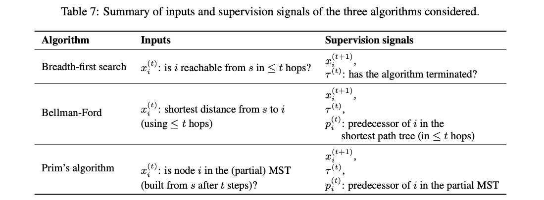
The performance of a curriculum learning strategy (as curriculum): here, BFS is learnt first in isolation (to perfect validation accuracy), followed by fine- tuning on Bellman-Ford. We find that this approach performs worse than learning both algorithms simultaneously, and as such we do not consider it in further experiments. So basically we should learn more algorithms simultaneously and exploiting the similarities between their respective subroutines whenever appropriate.
EXTRA (IGNORE IF NOT INTERESTED): In the Appendix B. of the paper authors give a theoretical reason why simultaneously learning may provide benefits in downstream task. Consider that for the same input \(x\), two different outcomes are \(y_A\) using algorithm \(A\) and \(y_B\) using algorithm \(B\). Now we imply that the two algorithms share some subroutines so the Conditional Mutual Information of the corresponding random variables \(x, y_A, y_B\) is \(I(Y_A;Y_B|X)\) can be expanded as \[I(Y_A;Y_B|X) = H(Y_A|X) - H(Y_A,Y_B|X)\] where \(H\) is the Shannon Entropy. Now from experiments we know that \(I(Y_A;Y_B|X)\) is positive thus \(H(Y_A|X) > H(Y_A,Y_B|X)\) therefore providing \(y_B\) upfront strictly reduces the information-theoretic uncertainty in \(y_A\), thus making it potentially more suitable for being learned by optimisation techniques.
Neural Execution Engines (Yan et al.)
Though the above two results are good, we see that one of the main challenge they face is the generalisation over larger datasets, this is the particular target that this paper achieves. They take several basic algorithms (selection sort, merge sort, Dijkstra’s algorithm for shortest paths) and express them in terms of a series of subroutines, as a software engineer would. Each subroutine represents a simple function, and can be composed with others to express the algorithm. In this way, we train neural networks to perform relatively simple tasks in a supervised manner, and obtain complex behaviors through composition.
They take the base Transformer and modify the masking mechanism. Simply stated, a neural execution engine (NEE) is a transformer that takes as input binary numbers and an encoding mask, and outputs either data values, a pointer, or both. The pointer can optionally be used to modify the mask the next time the NEE is invoked. There are some ideas that are new here and noted below:
- Bitwise Embedding: It is used where given an embedding vector \(v_i\) for each bit \(i\), for an \(n\)-bit input vector \(x\), we would compute \(\hat{x} = \sum_{i=1}^{n} x_i v_i\). For example, \(emb(1001) = v_0+v_3\) . The other two special tokes are the start \(s\) and end \(e\) tokens.
- Conditional Masking: In this we use the output pointer of the decoder to modify the mask for a subsequent call of the encoder. In this way, the inputs represent a memory state, and the mask represents a set of pointers into the memory. The binary mask \(M\) has value \(0\) where to focus and \(1\) where not to focus. The input mask \(b\) and output \(o\) of the transformer result in mask for next state as \(\hat{b} = xor(b, o)\). It is sufficient for the algorithms given here.
- Encoding Independent Inputs: The function must operate on a sequence of inputs, but where subsets of the inputs can be treated independently.
- Encoding Dependent Inputs: If we receive two sub sequences we merge using \(e\) token as \(\{ [a,b];[c,d] \} \rightarrow [a, b, e, c, d, e] \) and the mask could become \([0, 0, 1, 0, 0, 1]\) and if we need to iterate over sub-sequences we could use \([0, 1, 1, 0, 1, 1]\).
- Decoding: In decoding we start with the start tag \(s\) and compute attention over encoder blocks and return a single value and/or pointer instead of sequence.

Seq2Seq style sorting when trained on sequences upto length 8. Thing to note is that despite heavy modifications the vanilla transformer is not really doing anything good.
Authors found that sorting random numbers was easier than sorting those with minor difference (eg. \(1\) and \(90\) vs \(53\) and \(54\)). The decoder uses a greedy decoding strategy. The outputs of the decoder are one-hot \(256\) dim vectors representing the unnormalized log-probabilities of the output numbers. Thus training data has 70% random numbers, 30% numbers with small differences. The reason was seen when authors focused on the attention in the last layer of the decoder the attention was proper for the first few numbers but went completely fuzzy for the later numbers as seen in the image below.

- Subroutine Level Traces (Selection Sort): Using this insight authors decided to increase teh supervision and break the problem in sub tasks which are more atomic than the previous paper. For example the task in selection-sort is to find the minimum of the list and that can be replaced with a neural network and to increase focus (attention only on required things), a mask was used to tell where it could attend.
- Recursive Subroutines (Merge Sort): In merge sort the list of the list is broken in two equal pieces till there is only one left and then they are joined iteratively, this is a recursive method as showin the image below. The NEE is able to learn merge sort with perfect strong generalization over long sequences (up to length 100). The NEE was trained to perform the computation underlying merge sort on sequences of length ≤ 8.
- Composable Subroutines (Shortest Path): After the success in recursive patterns the next question was whether it would learn something that was made up of many different pieces.

Subroutine Level Traces in Selection Sort.
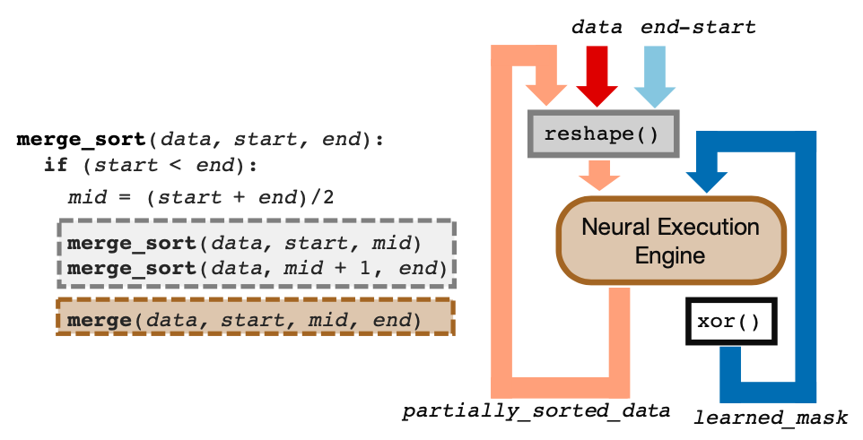
Recursive Subroutine in Merge Sort.
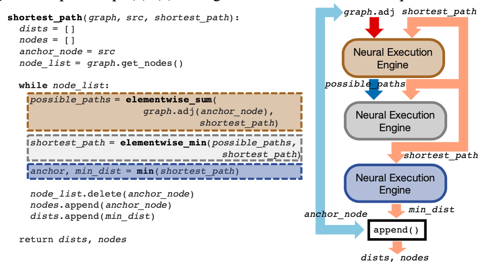
Djikstra's Algorithm to NEE Architecture.
In order to see how the learning happened the emebddings for the numbers was passed through PCA, we can see that highly structured understanding of number system by the system. You can see that in the image below.
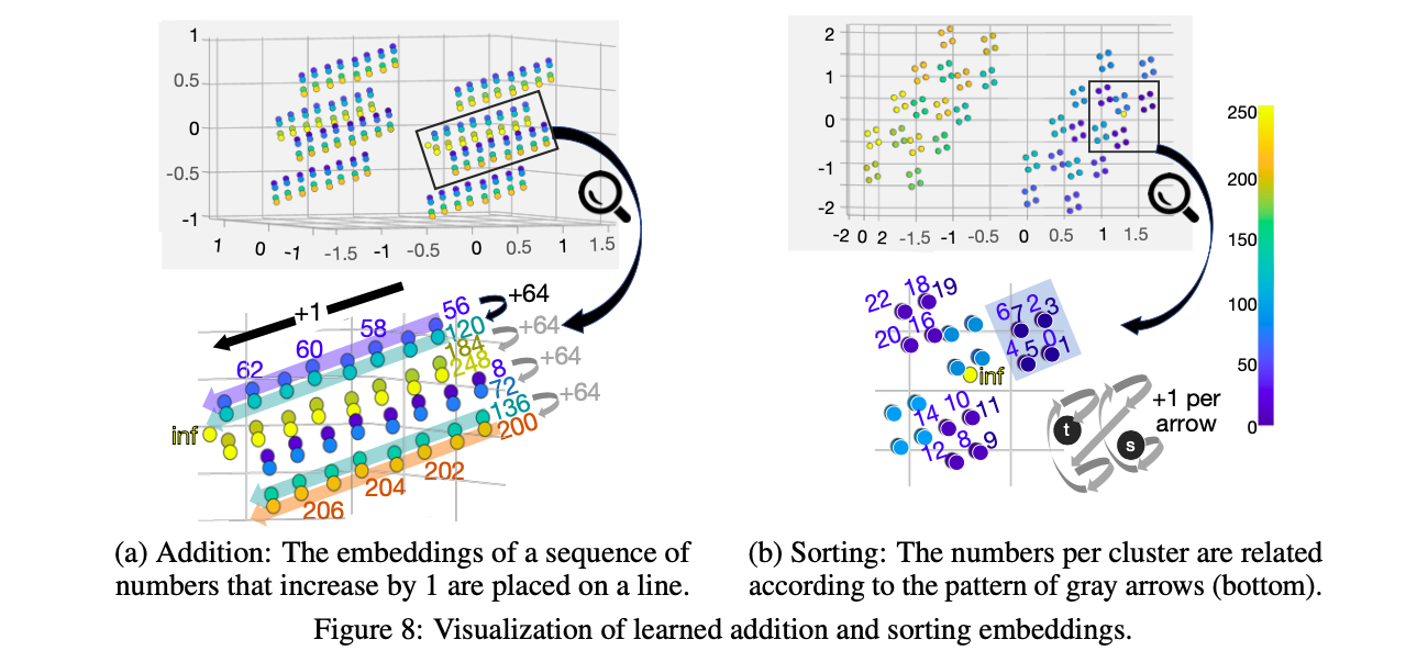
Model shows understanding of the number system

Model showed unparalled results by learning what to actually do. All seven images above are from here
Conclusion
This was probably the biggest note-taking thing I have done is some time, and it solves a variety of doubts I had on graph neural networks and introduced me to the theory of something I did not know was called "Neural Algorithm Execution" where the neural network learns programs. The couple of interesting points from the reading was this:
- Graph networks that closely resemble the existing algorithsm work better, so find the algorithm and get the simples network for it.
- Microscopic networks trained via intense supervision tend to learn much better and scale much better
Total Reading List
This is the list of all the papers in the above notes and some more, in case you are interested in the details.
- GNNExplainer: Generating Explanations for Graph Neural Networks (link)
- Nerual GPUs Learn Algorithms (link)
- Neural Random Access Machines (link)
- Neural Execution Engines (link)
- Neural Execution of Graph Algorithms (link)
- What Neural Networks can reason about? (link)
- Neural Turing Machines (link)
- An Efficient Graph Convolutional Network Technique for the Travelling Salesman Problem (link)
- Simplifying Graph Convolutional Network (link)
- On Graph Classification Networks, Datasets and Baselines (link)
- Pitfalls of Graph Neural Network Evaluation (link)
- Deep Graph Infomax (link)